TL;DR: A quick look at the binomial and negative binomial distributions through the lens of basketball shooting drills.
A friend and I were doing basketball shooting drills. To make things interesting, we bet on each round: the loser paid a dollar for every shot they lost by. For the first drill we took 30 shots. E.g. if I made 16 and he made 14, I’d win $2. For the next drill you shot until you made 15, with the loser paying a dollar for each extra miss. So if I took 27 shots to make my 15 (12 misses) and it took them 31 (16 misses), I’d win $4.
If we each shoot 50%, both games have the same expected outcome: 30 shots each, 15 for 30, and the bet’s a wash. But while the expected values match, the spread of outcomes is quite different.
Scenario 1: difference of binomial distributions
The distribution of outcomes for the first scenario can be modeled as the difference of two binomial distributions. To unpack this a little: the chance of making a single shot can be represented by what’s termed a bernoulli distribution1, which just assigns a probability to each of the two outcomes (make or miss). A binomial distribution then gives the distribution of successes2 across some number of bernoulli trials3. E.g. given a 50% chance of making each shot and 30 attempts, what’s the chance you make 0, 1, 2, … up to 30 shots.
Here’s what that distribution looks like for a 50% shooter taking 30 shots:
library(tidyverse)

tibble(makes = 0:30) |>
  mutate(probability = dbinom(makes, 30, 0.5)) |>
  ggplot(aes(x = makes, y = probability))+
  geom_col()+
  theme_bw()+
  scale_y_continuous(labels = scales::percent)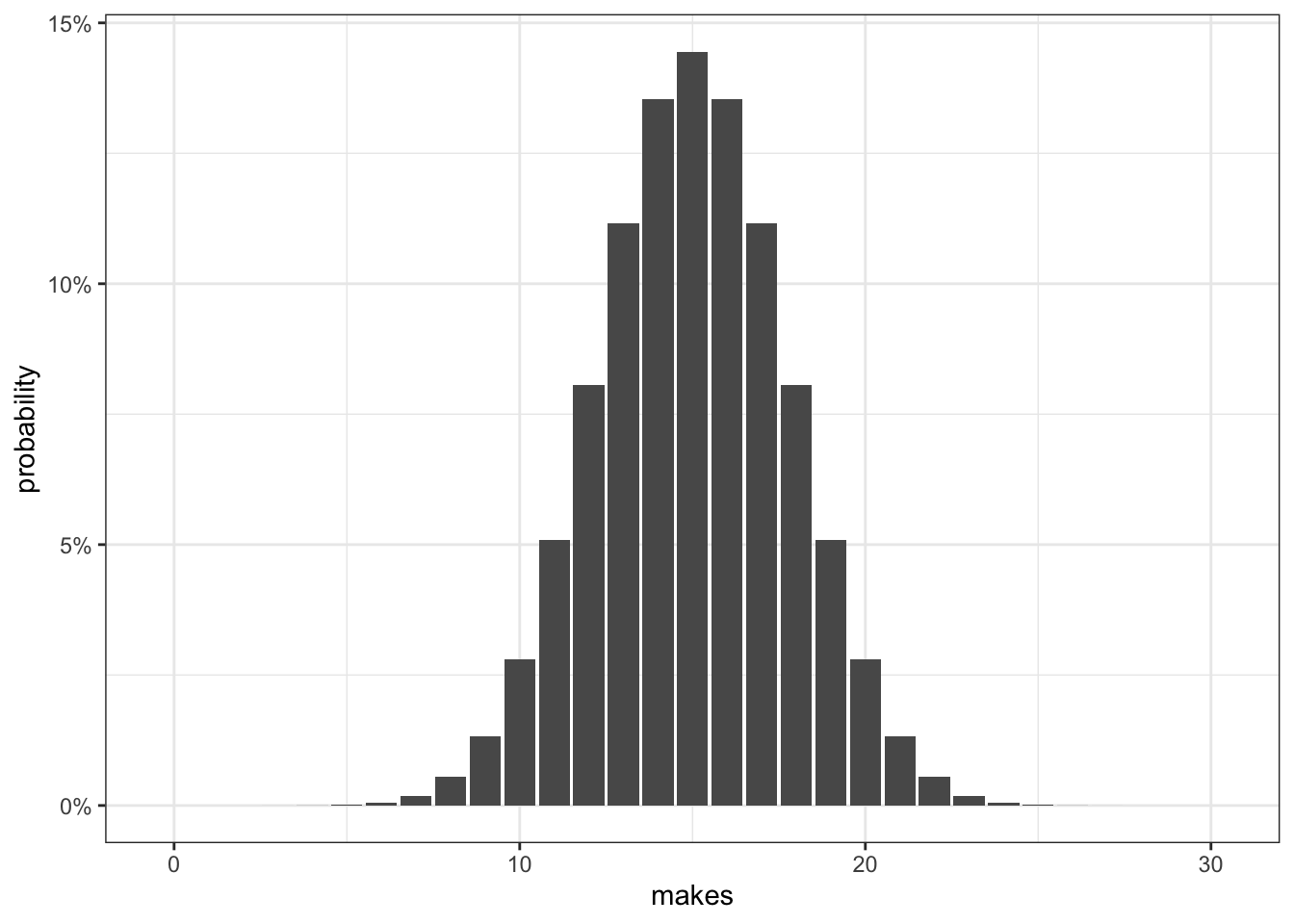
However I care about modeling pay-outs, i.e. the distribution of the difference in makes between me and my friend. In this simple case you could derive that distribution analytically4, but often your situation is too complicated to derive, so instead you simulate from the underlying components. Each round here is just the difference of two binomial distributions (each 30 shots at 50%). I’ll run this a million times and look at the distribution of payouts5:
set.seed(123)
# simulate a million rounds of 30 v 30 shots
output <- tibble(outcomes = rbinom(1000000, 30, 0.5) - rbinom(1000000, 30, 0.5))

output |>
  count(outcomes) |>
  mutate(prop = n / sum(n)) |>
  ggplot(aes(x = outcomes, y = prop))+
  geom_col()+
  theme_bw()+
  scale_y_continuous(labels = scales::percent)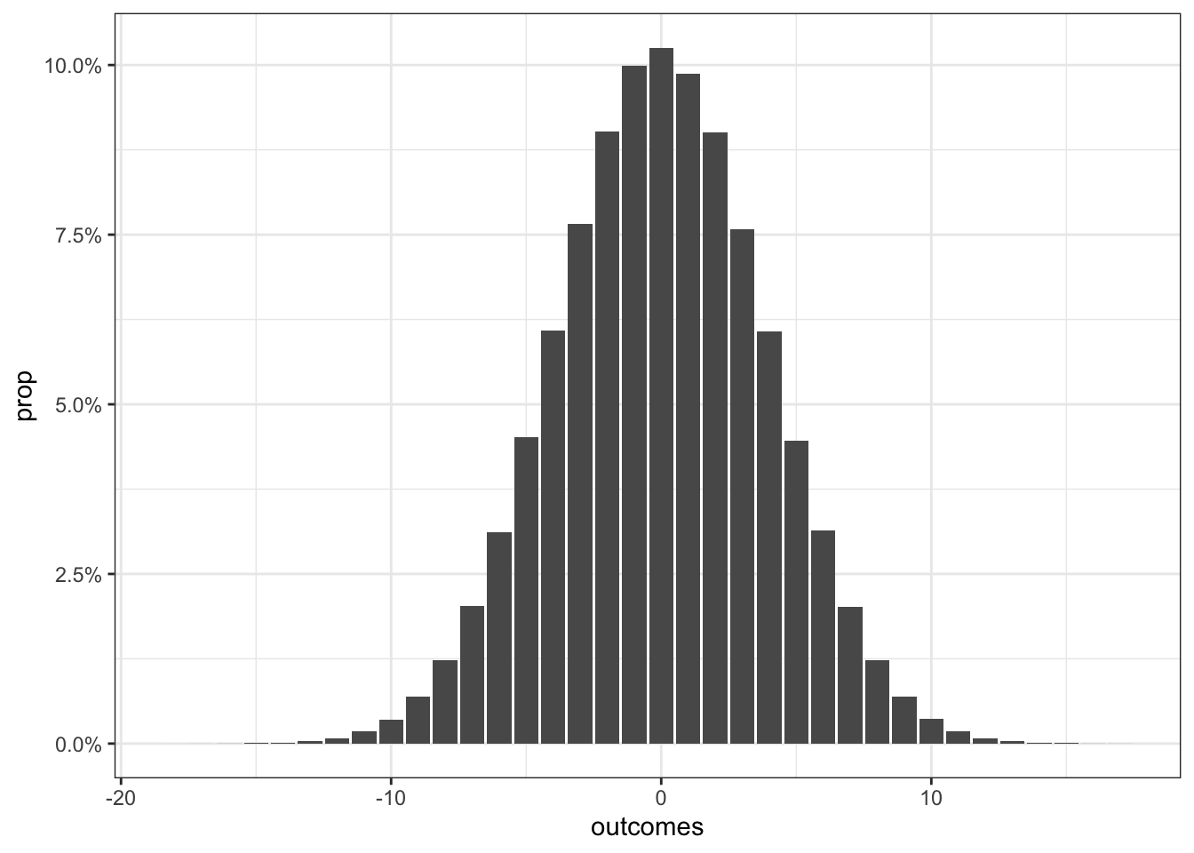
For spread, let’s look at the magnitude of payouts irrespective of who wins.
output_abs <- output |> mutate(outcomes_abs = abs(outcomes))

output_abs |>
  count(outcomes_abs) |>
  mutate(prop = n / sum(n)) |>
  ggplot(aes(x = outcomes_abs, y = prop))+
  geom_col()+
  theme_bw()+
  scale_y_continuous(labels = scales::percent)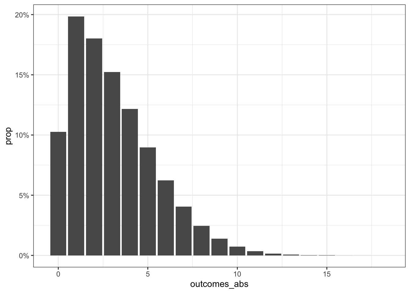
The typical (50th percentile) outcome is someone winning by three shots; the 90th percentile is six.
output_abs |>
  with(quantile(outcomes_abs, c(0.5, 0.9)))
## 50% 90%
## 3 6Scenario 2: difference in negative binomial distributions
In our second scenario we no longer have a fixed number of shots and an uncertain number of makes – we’ve fixed the makes at 15 and want the distribution of misses accumulated on the way there. We’re asking the inverse, or negative, of the earlier question, so perhaps it’s no surprise the relevant distribution is called the negative binomial. It too can be thought of as a series of bernoulli trials, but now we keep shooting until we hit a target number of makes, counting the failures along the way678.
Here’s the distribution of misses on the way to 15 makes for a 50% shooter.
tibble(misses = 0:50) |>
  mutate(probability = dnbinom(misses, 15, 0.5)) |>
  ggplot(aes(x = misses, y = probability))+
  geom_col()+
  theme_bw()+
  scale_y_continuous(labels = scales::percent)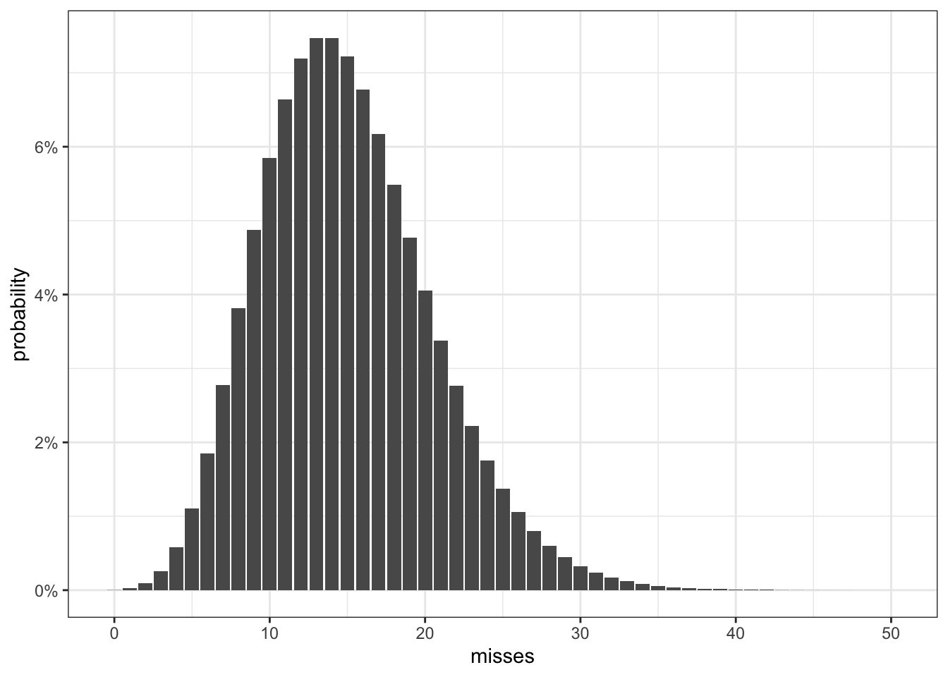
A couple things to notice:
- it’s wider than our initial binomial distribution – the variance here is 309 vs 7.510 for the binomial.
- it’s right skewed11.
So it’s not surprising that simulating the difference of two negative binomials also shows a wider spread:
set.seed(123)
nb_output <- tibble(outcomes = rnbinom(1000000, 15, 0.5) - rnbinom(1000000, 15, 0.5))

nb_output |>
  count(outcomes) |>
  mutate(prop = n / sum(n)) |>
  ggplot(aes(x = outcomes, y = prop))+
  geom_col()+
  theme_bw()+
  xlim(c(-40, 40))+
  scale_y_continuous(labels = scales::percent)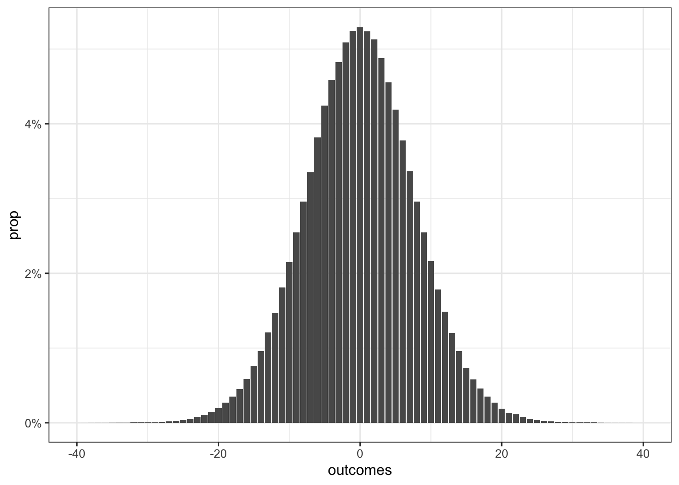
In terms of magnitude of payouts:
nb_output_abs <- nb_output |> mutate(outcomes_abs = abs(outcomes))

nb_output_abs |>
  count(outcomes_abs) |>
  mutate(prop = n / sum(n)) |>
  ggplot(aes(x = outcomes_abs, y = prop))+
  geom_col()+
  theme_bw()+
  xlim(c(0, 40))+
  scale_y_continuous(labels = scales::percent)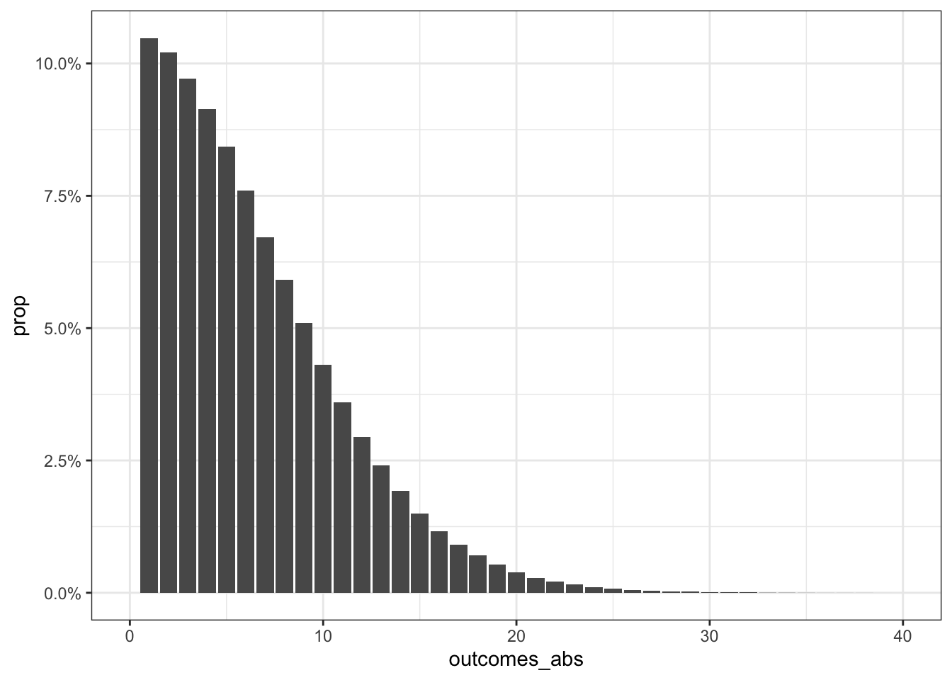
Our typical payout is now $5 and our 90th percentile payout is $13 (compared to $3 and $6 respectively in our first game).
nb_output_abs |>
  with(quantile(outcomes_abs, c(0.5, 0.9)))
## 50% 90%
## 5 13So if you hold the successes constant you can expect larger payouts between rounds in our second game1213.
Which game should you play if you’re better?
Say you have an edge on your friend. Which game is better for you?
Let’s plot the expected value and standard deviation of payouts as your friend’s shooting percentage drops from 50% to 40%.
diffs_of_dists <- function(prob2, prob1 = .5, dist = rbinom, n = 30, size = 1000000){
  dist(size, n, prob1) - dist(size, n, prob2)
}

game_stats <- map_dfr(seq(.40, .50, by = 0.01), function(prob_friend){
  binom_diffs <- diffs_of_dists(prob_friend)
  # in scenario 2 fewer misses is better, so flip the sign to get *your* payout
  nbinom_diffs <- -diffs_of_dists(prob_friend, n = 15, dist = rnbinom)

  tibble(
    friend_shooting_pct = prob_friend,
    game = c("scenario 1: fixed shots", "scenario 2: shoot until 15 makes"),
    expected_payout = c(mean(binom_diffs), mean(nbinom_diffs)),
    sd_payout = c(sd(binom_diffs), sd(nbinom_diffs))
  )
})

game_stats |>
  pivot_longer(c(expected_payout, sd_payout)) |>
  mutate(name = ifelse(name == "expected_payout", "expected payout", "standard deviation of payout")) |>
  ggplot(aes(x = friend_shooting_pct, y = value, colour = game))+
  geom_line()+
  facet_wrap(~name, ncol = 1, scales = "free_y")+
  expand_limits(y = 0)+
  theme_bw()+
  theme(legend.position = "bottom")+
  scale_x_continuous(labels = scales::percent, breaks = c(.40, .45, .50))+
  scale_y_continuous(labels = scales::dollar, breaks = seq(0, 10, by = 2))+
  labs(x = "friend's shooting percentage", y = NULL)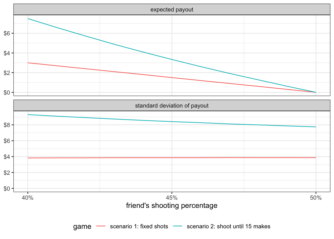
Scenario 2 has the better expected payout but more uncertainty – and its uncertainty grows with the skill gap, whereas scenario 1’s variability stays about the same either way.
So the two games are only “the same” on average. The data generating process doesn’t just set what you expect to win – it also sets the spread of what actually happens and how that spread moves with the skill gap. Pick your game accordingly.
Appendix
Hypothesis tests on observational data
The two games can also mess with a statistician using observational data with no control of sample size. Pretend someone at the community center likes to watch players doing shooting drills and use the observational data to run hypothesis tests on whether they’re equally skilled. The observer doesn’t control the games – they just analyze whatever shots happen. Let’s simulate type 1 (detects a difference when there isn’t one) and type 2 (misses a difference when there is one) errors under a few scenarios.
One tweak first: we’ll have the players run longer versions of both games – 100 shots in the fixed game, shoot until 50 makes in the other14.
The observer would most likely use:
- difference of proportions z test
- chi-square test
- fisher’s exact test
I’ll simulate the outputs from each.
run_tests <- function(makes, misses){
  shot_table <- rbind(makes, misses)

  tibble(
    `z test` = prop.test(makes, makes + misses, correct = FALSE)$p.value,
    `chi-square test` = chisq.test(shot_table)$p.value,
    `fisher's exact test` = fisher.test(shot_table)$p.value
  )
}

simulate_tests <- function(prob1, prob2, game, n_sims = 10000){
  map_dfr(1:n_sims, function(sim){
    if(game == "scenario 1"){
      makes <- c(rbinom(1, 100, prob1), rbinom(1, 100, prob2))
      misses <- 100 - makes
    } else {
      misses <- c(rnbinom(1, 50, prob1), rnbinom(1, 50, prob2))
      makes <- c(50, 50)
    }
    run_tests(makes, misses)
  }) |>
    summarise(across(everything(), ~mean(.x < 0.05))) |>
    mutate(game = game, .before = 1)
}

set.seed(123)
bind_rows(
  simulate_tests(0.5, 0.5, "scenario 1") |> mutate(skill = "equal (both 50%)", .before = 1),
  simulate_tests(0.5, 0.5, "scenario 2") |> mutate(skill = "equal (both 50%)", .before = 1),
  simulate_tests(0.5, 0.4, "scenario 1") |> mutate(skill = "different (50% v 40%)", .before = 1),
  simulate_tests(0.5, 0.4, "scenario 2") |> mutate(skill = "different (50% v 40%)", .before = 1)
) |>
  mutate(game = ifelse(game == "scenario 1", "scenario 1: fixed 100 shots", "scenario 2: shoot until 50 makes")) |>
knitr::kable()| skill | game | z test | chi-square test | fisher’s exact test |
|---|---|---|---|---|
| equal (both 50%) | scenario 1: fixed 100 shots | 0.0565 | 0.0401 | 0.0401 |
| equal (both 50%) | scenario 2: shoot until 50 makes | 0.0482 | 0.0351 | 0.0401 |
| different (50% v 40%) | scenario 1: fixed 100 shots | 0.3163 | 0.2671 | 0.2671 |
| different (50% v 40%) | scenario 2: shoot until 50 makes | 0.3274 | 0.2794 | 0.3007 |
The table shows the proportion of rounds where each test flagged a skill difference: for “equal” rows that’s the type 1 error rate (should be near our 5% significance level), for “different” rows it’s the power of the test (the complement of the type 2 error rate).
With equal players all three tests hold up in either game (z close to nominal, chi-square and fisher’s exact a touch conservative). But when there is a skill gap, every test is more likely to catch it in the shoot-until game. Same shooters, same tests but the observer reaches different conclusions at different rates depending on which game happened to be played.
The culprit is mostly sample size: reaching 50 makes at a 40% clip takes ~125 shots vs the fixed 100, so the shoot-until game generates more data on the weaker shooter. With observational data your sample is often at the whims of the unknown data generating process which can impact your conclusions in observational studies15.
though this can also be thought of as a special case of a binomial distribution where number of rounds is equal to 1.↩︎
In our case, given the probability of making each shot and the number of attempts, its probability mass function assigns a probability to each possible number of makes.↩︎
I.e. rounds of selecting from a bernoulli distribution.↩︎
using fancy math and convolution↩︎
I’m pretending we played a million rounds and showing the proportion of rounds that land in each payout bucket. Downsides of simulation: it can be slow, and it can struggle to accurately capture the tails of the distribution. E.g. if you care about a 1 in 100,000 outcome, a simulation of a million rounds will only produce a handful of draws that far out, so the simulated tail is noisy. In those cases you can apply methods that smooth information across the rare outcomes (or lean on analytic results) to get a better estimate of the tails.↩︎
Equivalently, you can think of it as a sum of geometric distributions: chop the sequence of shots at each make and the misses between consecutive makes follow a geometric distribution, so our negative binomial is just the sum of 15 geometrics. This sum-of-independent-pieces view is also why the normal approximation discussed later works.↩︎
Here’s a video with a little more detail on these distributions and the relation between them: https://www.youtube.com/watch?v=BPlmjp2ymxw↩︎
Conveniently, R’s
dnbinom()andrnbinom()are parameterized in terms of the number of failures before hitting a target number of successes – which maps exactly onto counting misses before 15 makes.↩︎(r * (1 - p)) / p^2 = (15 * 0.5) / 0.5^2 = 30↩︎
n * p * (1 - p) = 30 * 0.5 * 0.5 = 7.5↩︎
I cut the chart at 50 misses but the distribution goes on to infinity.↩︎
You could actually skip the simulations here: both payout distributions are approximately normal (a binomial is a sum of bernoulli trials, a negative binomial is a sum of geometrics, so the CLT applies – and differencing two identical copies cancels the negative binomial’s right skew). Scenario 1 is roughly N(0, 2 * n * p * (1 - p)) and scenario 2 roughly N(0, 2 * r * (1 - p) / p^2), and if you hold the expected number of shots equal (n = r / p) the ratio of the standard deviations works out to exactly 1/p. At 50% shooting the shoot-until game has exactly double the spread.↩︎
This roughly doubled spread isn’t an artifact of double counting: in the first game paying on the difference in makes is the same as paying on the difference in misses (shots are fixed at 30, so every extra make is exactly one fewer miss). Both games are settling-up on misses, the shoot-until-15 game just genuinely has about twice the spread. You can see the same relationship in the expected (absolute) payouts: $6.12 for the shoot-until-15 game vs $3.08 for fixed shots.↩︎
At the shorter lengths from earlier, the counts are small enough that these tests all get a bit conservative and noisy, which muddies the comparison we care about.↩︎
E.g. if you only took the first 50 observations then it doesn’t matter which game was being played – the first 50 shots of either game are just the same coin flips, since a stopping rule can’t affect shots taken before it kicks in:
z_pvalue <- function(makes1, makes2, n = 50){
  prop.test(c(makes1, makes2), c(n, n), correct = FALSE)$p.value
}

# play out a shoot-until-50-makes game, but only score the first 50 shots
first_50 <- function(prob){
  shots <- rbinom(500, 1, prob)
  sum(shots[1:50])
}

set.seed(123)
map_dfr(1:10000, function(sim){
  tibble(
    `first 50 of fixed 100` = z_pvalue(rbinom(1, 50, 0.5), rbinom(1, 50, 0.4)),
    `first 50 of shoot until 50` = z_pvalue(first_50(0.5), first_50(0.4))
  )
}) |>
  summarise(across(everything(), ~mean(.x < 0.05))) |>
  knitr::kable()
↩︎first 50 of fixed 100 first 50 of shoot until 50 0.186 0.1874