TLDR: FiveThirtyEight’s forecasts of NBA playoff berths seem to hold-up OK against betting markets. If you trust them, you should consider betting against the Lakers right now.
In The Virtues and Vices of Election Prediction Markets Nate Silver explains why FiveThirtyEight generally should not beat the market:
“The general question of whether FiveThirtyEight ought to be better than prediction and betting markets is an interesting one. I am far from an efficient-market hypothesis purist, but markets are tough to beat in most circumstances. Furthermore, the FiveThirtyEight forecasts are public information, and bettors can use our forecasts along with those of our competitors to calibrate their estimates of the outcomes.”
FiveThirtyEight does more with their forecasts than just predict outcomes. Their forecasts provide the foundation of their data journalism covering trends in sports and politics. We should expect FiveThirtyEight’s forecasts to make some tradeoffs between optimizing for performance and being interpretable1. Their NBA model is based on a blend of team and individual player performance and is designed with various linear constraints in place that make it explainable to the public (see: How Our NBA Predictions Work).
However performance costs shouldn’t be too high. Afterall, trust in FiveThirtyEight’s explanations is in large part dependent on their models’ predictive power.
The public should root for forecasters like FiveThirtyEight
Where betting markets exist, public forecasts like FiveThirtyEight’s add information into the system and can help markets reach more efficient prices. Where markets don’t exist, we are limited to the power of such forecasting processes – be it government impact assessments, weather forecasts, disease modeling, … – society gains as predictive power improves2.
NBA Playoffs and the Lakers
I was struck the other day by a substantial difference between FiveThirtyEight and the betting markets in their outlook on the Lakers. I remarked that FiveThirtyEight should add an additional point of comparison to their documentation of How Good are FiveThirtyEight Forecasts3.
I get betting markets will be better but by how much?
— Bryan Shalloway (@brshallo) December 6, 2021
For NBA predictions I feel like I'll see stuff wildly out-of-touch with betting markets (eg lakers 27% to make playoffs on 538 but -460 on betting markets) and I don't know what to think.
I could not (immediately) find any performance comparisons beween betting markets and FiveThirtyEight forecasts of NBA playoffs, so pulled the data and wrote this post4.
Spoiler on Analysis: Turns out, FiveThirtyEight holds-up pretty well.
Data Prep
Scraping Betting Markets
I scraped historical betting lines and which teams actually made the playoffs each season from the “Archived NBA Futures Odds” section of Sports Odds History5. The Sports Odds History website is constructed in a way that makes it relatively straight-forward to scrape the requisite information.
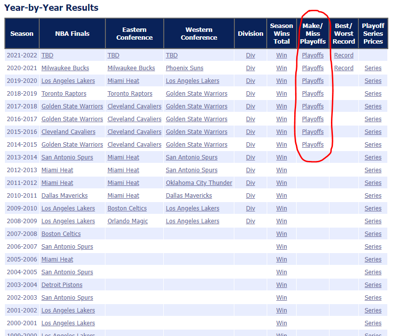
The webpage for each season has a (mostly) consistent table structure and associated date of archive.
Each season has a consistent URL (with only the season year changing).

Steps
- Create table with URL’s to scrape
- For each URL repeat steps 3 to 6
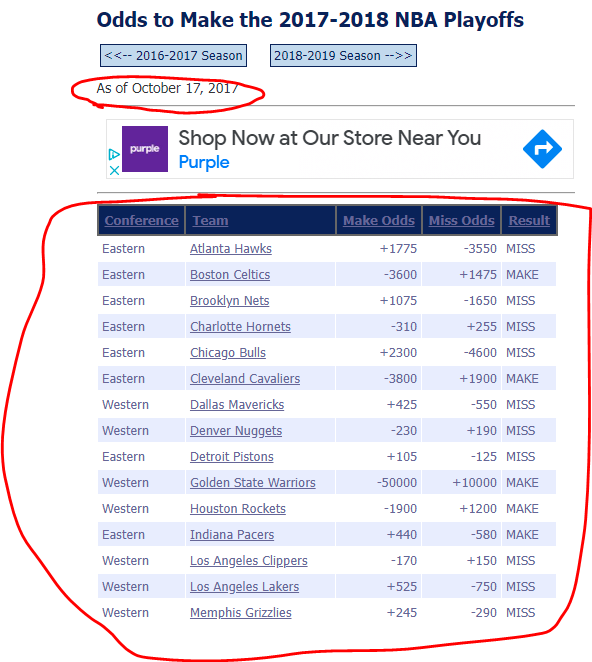
- Scrape table containing Teams, betting odds, and outcomes6
- Convert from payouts to odds (e.g. +400 becomes 0.25)
- Tables contain the betting odds of both “making the playoffs” and “missing the playoffs”7. I took the average of the implied odds of making the playoffs between both columns (“make” and inverse of “miss”). This might be generous to the betting markets but likely gets at a closer estimate of where they actually expect the odds to be.
- Scrape date archived and join to table
- Bind data from all scraped pages / seasons together
- Convert from odds to probability (e.g. 4:1 becomes 80%)
Load packages and helper functions
# Load packages
library(tidyverse)
library(rvest)
library(gt)
library(broom)

# Helper functions
# Some of the tables had the lines represented as character strings like "+400"
# "-300". This converts those to a numeric type (if they're not  already).
odds_to_numeric <- function(x){
  if(is.numeric(x)) return(x)
  sign <- str_sub(x, 1, 1)
  sign <- case_when(sign == "-" ~ -1,
                    sign == "+" ~ 1)
  x_dbl <- str_sub(x, 2) %>% as.double()
  x_dbl * sign
}

# -400 would be converted to 4, +400 to 0.25
line_to_odds <- function(x){
  positive <- sign(x) == 1
  abs_x <- abs(x)
  case_when(positive ~ 100 / abs_x ,
            !positive ~ abs_x / 100)
}

odds_to_prob <- function(odds){
  odds / (1 + odds)
}
I’ve labeled each respective # step in the code sections below.
Step 1
# step 1
scrape_urls <- tibble(start_yr = 2014:2020, end_yr = 2015:2021) %>%
  mutate(yr = paste0(start_yr, "-", end_yr),
         urls = glue::glue(
           "https://www.sportsoddshistory.com/nba-win/?y={yr}&sa=nba&t=post&o=s",
           yr = yr
         ))


scrape_urls %>%
gt::gt()| start_yr | end_yr | yr | urls |
|---|---|---|---|
| 2014 | 2015 | 2014-2015 | https://www.sportsoddshistory.com/nba-win/?y=2014-2015&sa=nba&t=post&o=s |
| 2015 | 2016 | 2015-2016 | https://www.sportsoddshistory.com/nba-win/?y=2015-2016&sa=nba&t=post&o=s |
| 2016 | 2017 | 2016-2017 | https://www.sportsoddshistory.com/nba-win/?y=2016-2017&sa=nba&t=post&o=s |
| 2017 | 2018 | 2017-2018 | https://www.sportsoddshistory.com/nba-win/?y=2017-2018&sa=nba&t=post&o=s |
| 2018 | 2019 | 2018-2019 | https://www.sportsoddshistory.com/nba-win/?y=2018-2019&sa=nba&t=post&o=s |
| 2019 | 2020 | 2019-2020 | https://www.sportsoddshistory.com/nba-win/?y=2019-2020&sa=nba&t=post&o=s |
| 2020 | 2021 | 2020-2021 | https://www.sportsoddshistory.com/nba-win/?y=2020-2021&sa=nba&t=post&o=s |
Steps 2-6
Custom scraping function:
scrape_nba_playoffs_odds <- function(url){

  css_selector_tbl <- "#content > div > table.soh1"

  html_page <- url %>%
    read_html()

  # step 3
  data <- html_page %>%
    html_element(css = css_selector_tbl) %>%
    html_table() %>%
    janitor::clean_names() %>%
    mutate(
      # step 4
      across(contains("odds"),
             list(dbl = ~odds_to_numeric(.x) %>%
                    line_to_odds())),
      # step 5
      make_odds_avg = (make_odds_dbl + 1 / miss_odds_dbl) / 2)

  html_kids <- html_page %>%
    html_element(css = "#content > div") %>%
    html_children() %>%
    html_text2()

  # step 6
  phrase_date <- "As of "
  date_taken <- html_kids %>%
    str_subset(phrase_date) %>%
    str_extract(glue::glue("(?<={phrase_date}).+")) %>%
    lubridate::mdy()

  data %>%
    mutate(forecast_date = date_taken) %>%
    # type varied between webpages so force to chr so can bind multiple...
    mutate(across(c(make_odds, miss_odds), as.character)) %>%
    relocate(forecast_date)
}
map() function to scrape_nba_playoffs_odds() on urls
# Step 2 (applies steps 3 through 6 on each URL)
scraped_urls <- scrape_urls %>%
  mutate(data = map(urls, scrape_nba_playoffs_odds))
Steps 7-8
odds_data_prepped <- scraped_urls %>%
  select(season = end_yr, data) %>%
  # step 7
  unnest(data) %>%
  arrange(desc(season)) %>%
  mutate(
    # step 8
    make_playoffs_bookies = odds_to_prob(make_odds_avg),
    result = ifelse(result == "MAKE", 1, 0)
    ) %>%
  select(season, forecast_date, team, result, make_playoffs_bookies) %>%
  mutate(team = str_extract(team, "(?<=[:blank:])[:alnum:]+$"))
Joining with FiveThirtyEight data
- All FiveThirtyEight NBA playoff forecasts were available in a .csv on github here.
- FiveThirtyEight updates their forecasts every day. For the archived betting market payouts there is only one day of odds for each season. I filtered FiveThirtyEight forecasts to just those days where I also had market data8.
- Joined FiveThirtyEight forecasts with market and outcome data.
- In a few instances market data was not available, in which case I also filtered out the corresponding FiveThirtyEight records.
Steps 9 to 12
# step 9
data_538 <- read_csv("https://raw.githubusercontent.com/fivethirtyeight/checking-our-work-data/master/nba_playoffs.csv")

bookies_538_joined <- data_538 %>%
  # step 10
  filter(forecast_date %in% unique(odds_data_prepped$forecast_date)) %>%
  select(season, forecast_date, team, make_playoffs_538 = make_playoffs) %>%
  # step 11
  left_join(odds_data_prepped, by = c("season", "team", "forecast_date")) %>%
  # step 12
  na.omit() %>%
  # mutate(make_playoffs_avg = (make_playoffs_538 + make_playoffs_bookies) / 2) %>%
  relocate(result, .after = team)
Resulting table for analysis (preview of 5 rows)
bookies_538_joined %>%
  head(5) %>%
  gt::gt() %>%
gt::fmt_number(decimals = 3, columns = c("make_playoffs_538", "make_playoffs_bookies"))| season | forecast_date | team | result | make_playoffs_538 | make_playoffs_bookies |
|---|---|---|---|---|---|
| 2020 | 2019-10-22 | Bucks | 1 | 0.995 | 0.976 |
| 2020 | 2019-10-22 | Timberwolves | 0 | 0.525 | 0.172 |
| 2020 | 2019-10-22 | Heat | 1 | 0.708 | 0.730 |
| 2020 | 2019-10-22 | Wizards | 0 | 0.214 | 0.122 |
| 2020 | 2019-10-22 | Hawks | 0 | 0.115 | 0.300 |
Analysis
FiveThirtyEight uses the Brier Score9 in their evaluations of model performance (see Some Do’s and Don’t’s For Evaluating Senate Forecasts)10. I mirrored this below.
Overall performance
### helper functions
t_test_playoffs <- function(df){
  df %>%
    with(t.test(make_playoffs_538, make_playoffs_bookies)) %>%
    broom::tidy() %>%
    select(
      estimate_diff = estimate,
      p.value,
      estimate_538 = estimate1,
      estimate_bookies = estimate2,
      starts_with("conf")
    )
}

gt_format_output <- function(df){
  df %>%
    rename_with(~str_replace(.x, "estimate_", "Brier.score.")) %>%
    gt::gt() %>%
    gt::fmt_number(columns = contains("."),
                   decimals = 3) %>%
    gt::tab_style(style = list(cell_text(weight = "bold")),
                locations = cells_body(columns = "p.value"))
}
###

bookies_538_joined %>%
  mutate(across(starts_with("make_playoffs"), ~(result - .x)^2)) %>%
  t_test_playoffs() %>%
gt_format_output()| Brier.score.diff | p.value | Brier.score.538 | Brier.score.bookies | conf.low | conf.high |
|---|---|---|---|---|---|
| 0.004 | 0.881 | 0.143 | 0.139 | −0.045 | 0.053 |
Performance by Season
bookies_538_joined %>%
  mutate(across(starts_with("make_playoffs"), ~(result - .x)^2)) %>%
  group_nest(season) %>%
  mutate(t_test = map(data, t_test_playoffs)) %>%
  select(-data) %>%
  unnest(t_test) %>%
gt_format_output()| season | Brier.score.diff | p.value | Brier.score.538 | Brier.score.bookies | conf.low | conf.high |
|---|---|---|---|---|---|---|
| 2016 | −0.029 | 0.635 | 0.142 | 0.172 | −0.153 | 0.094 |
| 2017 | 0.050 | 0.268 | 0.159 | 0.109 | −0.040 | 0.140 |
| 2018 | 0.007 | 0.887 | 0.127 | 0.120 | −0.095 | 0.109 |
| 2019 | 0.019 | 0.793 | 0.204 | 0.185 | −0.127 | 0.166 |
| 2020 | −0.029 | 0.502 | 0.082 | 0.111 | −0.114 | 0.057 |
The p-values from the quick t-tests above suggest no statistically significant difference in performance between betting markets and FiveThirtyEight11.
How much does FiveThirtyEight differ from markets?
Overall performance may be similar even when individual forecasts are quite different. Circling back to the start of NBA Playoffs and the Lakers, what got me writing was noticing FiveThirtyEight’s divergence from the betting markets in their recent view of the Lakers’ playoff chances.
At -460 the markets had an implied probability of the Lakers making the playoffs of ~82%12. FiveThirtyEight’s forecast of 27% means a difference of ~55 percentage points (ppt)13.
Is this difference atypical?
Across five seasons of data (145 observations), the correlation coefficient was 0.92 (strong correlation). The average difference between FiveThirtyEight and betting markets was ~10 percentage points.
bookies_538_joined %>%
  mutate(diff = abs(make_playoffs_538 - make_playoffs_bookies)) %>%
  # summarise(mean_diff = mean(diff)) %>%
  with(t.test(diff)) %>%
  broom::tidy() %>%
  select(avg_abs_ppt_diff_538_bookies = estimate, contains("conf")) %>%
  gt::gt() %>%
  gt::fmt_number(columns = everything(),
decimals = 3)| avg_abs_ppt_diff_538_bookies | conf.low | conf.high |
|---|---|---|
| 0.097 | 0.081 | 0.113 |
A difference of 55 ppt is bigger than any I saw in the historical data. The closest was 48 ppt14:
bookies_538_joined %>%
  mutate(make_playoffs_diff = abs(make_playoffs_538 - make_playoffs_bookies)) %>%
  arrange(desc(make_playoffs_diff)) %>%
  head(1) %>%
  gt::gt() %>%
  gt::fmt_number(columns = contains("make_playoffs"),
decimals = 3)In the Appendix I give some Potential Reasons for the Difference, though on its surface 55 ppt does seem like a historically large disagreement between FiveThirtyEight and the betting markets.
Closing Thought
Given the (apparent) parity in performance between FiveThirtyEight and the betting markets, the Lakers’ playoff odds are especially unclear. I can’t just write-off FiveThirtyEight as I’d been tempted to do.
When I see big differences i get tempted to write-off 538.
— Bryan Shalloway (@brshallo) December 6, 2021
But maybe it's just different but still meaningful (even if less performative at margins).
I don't look at it systematically enough to know (so why another comparison point–eg betting markets–would be helpful).
For the reasons given in the Introduction I would still lean towards trusting the betting markets15 but the current payout on draft kings of $450 on a $100 bet of the Lakers not making the playoffs is an intriguing opportunity that perhaps deserves a closer look16.
Appendix
Potential Reasons for the Difference
Some reasons why the observed 55 ppt difference in expectations between FiveThirtyEight and betting markets may not be as extreme as it seems:
- My historical data is looking at individual time-point comparisons at just one point for each season – perhaps betting markets and FiveThirtyEight vary more from one another at different points in the year than those at the points I have..
- Market odds (according to Sports Odds History) are archived come from BetMGM. I don’t know where I was looking when I saw the -460 odds on the Lakers. Each betting market is different and may have different levels of covariation with FiveThirtyEight’s forecasts.
- I was looking at just the “odds of making the playoffs” not the average of that with the inverse of “odds to miss the playoffs” as I did in step 5 of Steps17.
- Changes in methodology of more recent forecasts may have made it depart more from betting markets compared to in prior years
Calculating percentiles of diff
Initially I’d planned on including the calculation of some percentiles of various differences in percentage points. Saved code from examples below.
one_off_diff <- 0.27 - odds_to_prob(line_to_odds(-460))

bookies_538_joined %>%
  mutate(diff = abs(make_playoffs_538 - make_playoffs_bookies)) %>%
  summarise(percentile_of_difference = sum(diff < one_off_diff) / n())

# Alternative approach for calculating one-off diff
ecdf_diffs <- bookies_538_joined %>%
  mutate(diff = abs(make_playoffs_538 - make_playoffs_bookies)) %>%
  with(ecdf(diff))

ecdf_diffs(one_off_diff)
Model based forecasts are also reproducible – compared to a market based prices which are produced collectively and can’t be reproduced per se by an individual building a model. FiveThirtyEight’s model also has the challenge of trying to be consistent/coherent e.g. make player ratings meaningful and useful in aggregating up to give team ratings.↩︎
Public forecasting organizations like FiveThirtyEight also help promote data literacy and inspire improved predictive practices↩︎
While I think betting markets would be an ideal comparison point, a comparison against something simple like, “the teams with the best record will at this point will make the playoffs” or “the teams that made it to the playoffs last year will make it this year” would also represent improved comparison points.↩︎
I did found some writeups reviewing other FiveThirtyEight forecasts.↩︎
Whether team actually made it to playoffs that season↩︎
You might expect these to be inverses of one another, but they actually are slightly different – the difference provides room for The House to make a profit.↩︎
So that the forecasts and betting markets being compared were created the same day.↩︎
Essentially the root mean squared error of the classification.↩︎
I’ve remarked in the past on the differences in their performance evaluation from methods used by more pure ML and kaggle people:
↩︎Why do @kaggle and more ML people use log loss but @FiveThirtyEight @superforecaster and more probabilistic forecasting sites lean towards Brier Score?
— Bryan Shalloway (@brshallo) December 9, 2021
(1/3)Other ways to segment this could be by make/miss playoffs, high/low forecasted probabilities, reviewing an ensemble of bookies and 538 forecasts… but I don’t really expect any of these to be interesting so I’ll leave it there… and give a hat-tip to FiveThirtyEight for not getting creamed by the betting markets.↩︎
Note that I’m just using the line for “make playoffs” in the above analysis I’d taken the average of the odds of “making the playoffs” and the inverse of “missing the playoffs”…↩︎
If you check today FiveThirtyEight is not quite so down on the Lakers but still are quite a bit compared to the betting markets.↩︎
In that case in the favor of FiveThirtyEight.↩︎
I would be surprised if, after looking at a larger swathe of data, the markets did not come-out significantly better than FiveThirtyEight. Though perhaps the magnitude of the difference may be small.↩︎
Maybe at some point in the future I’ll review hypothetical outcomes of various strategies, e.g. ensembling, or betting in cases of high-levels of divergence between forecasts.↩︎
This would make the betting market odds seem more aggressive.↩︎