Part 1 of my series of posts on building prediction intervals used data held-out from model training to evaluate the characteristics of prediction intervals. In this post I will use hold-out data to estimate the width of the prediction intervals directly. Doing such can provide more reasonable and flexible intervals compared to analytic approaches¹.

This post is not required for understanding part three of the series: Quantile Regression Forests for Prediction Intervals. However this post assumes you have already read Part 1, Understanding Prediction Intervals ²:

I do not re-explain terms such as coverage and interval width (or relative measures) – which are discussed thoroughly in the section on Reviewing Prediction Intervals.
I do not reintroduce measures, figures, or chart types that were shown in the prior post.
I continue using Ames, Iowa home sale prices as my example dataset.

This post was largely inspired by topics discussed in the Prediction intervals with tidymodels, best practices? Rstudio Community thread.

Update

I copied most of the code referenced at gists in this post to the spin package. The workboots package by Mark Rieke is essentially the same thing³ but is available on CRAN. I also created a placeholder spinach where I may do some future work…

{spinach} – Simulating Prediction INtervals And CHance – a #tidymodels #tidyverse friendly📦for a general interface to simulating uncertainty of predictions.

Only a placeholder with a link to a prototype right now but hoping to start on soon: https://t.co/YpipdO5f1u #rstats pic.twitter.com/de2A4Z6WiD
— Bryan Shalloway (@brshallo) April 1, 2022

Rough Idea

Compared to analytic approaches, estimating sources of uncertainty through simulation has the advantage of…

relying on fewer model assumptions to still produce reasonable measures of uncertainty (though still generally requires that your model’s errors are iid).
can be applied to (essentially⁴) any model type⁵.

Approach:

The simulation based technique I walk through will take resamples of the data and generate separate distributions for what can be loosely thought of as:

the uncertainty due to model estimation
the uncertainty due to the sample

These will then be combined to produce an overall measure of uncertainty for the prediction⁶.

Inspiration

Dan Saattrup Nielsen also wrote a series of posts on prediction intervals. My approach here is mostly taken from the one he describes in Boostrapping prediction intervals. His approach is encoded in python whereas mine is in R for a tidymodels based set-up⁷. (In the Appendix, I describe and link to an implementation of an Alternative Procedure With CV that is influenced by suggestions from Max Kuhn.)

Dan’s post provides more precise symbolic representations as well as more figures showcasing results and advantages of simulation based approaches, e.g.

Example of more sensible handling of non-normality of errors, from Dan Saattrup’s excellent post Bootstrapping prediction intervals

The Appendix provides links from the web to Other Examples Using Simulation.

Procedure

Given the model training dataset with n number of observations…

Build b number of models using b bootstrap resamples on the training dataset (default of b is the square root of n)⁸.
Use the 0.632+ rule for blending errors from analysis and assessment sets⁹ (based on amount of overfitting in analysis set) and create a distribution of residuals evenly spaced across quantiles of length n – represents distribution for the uncertainty due to the sample.

Given an observation (or set of observations) you would like to produce prediction intervals for…

For each new observation, produce a prediction using all of the b models created in step 1.
Take the difference between each model’s prediction (from step 3) and the mean of all model predictions – the resulting b differences for each observation provides the distribution for the variability due to model estimation at each point.
For each observation, repeatedly sample from “residuals” (step 2) and “model error / differences” (step 4) and add together – do this h times (with replacement) OR create all possible combinations from step 2 and step 5. Rather than h, the latter approach will produce a distribution composed of n x b elements¹⁰ for each new observation (default behavior¹¹).
Pull quantiles (from the distribution created in step 5) according to the desired level of coverage of your intervals – e.g. 0.05 and 0.95 for a 90% prediction interval.

See gist for documentation on implementation.

Example

The initial set-up (load packages, load data, set pre-processing recipe, model specification) is the same as in the Providing More Than Point Estimates section of part 1. The code below is being sourced and printed from that post’s .Rmd file.

Load packages:

library(tidyverse)
library(tidymodels)
library(AmesHousing)
library(gt)

# function copied from here:
# https://github.com/rstudio/gt/issues/613#issuecomment-772072490 
# (simpler solution should be implemented in future versions of {gt})
fmt_if_number <- function(..., digits = 2) {
  input <- c(...)
  fmt <- paste0("%.", digits, "f")
  if (is.numeric(input))   return(sprintf(fmt, input))
  return(input)
}

Load data:

ames <- make_ames() %>% 
  mutate(Years_Old = Year_Sold - Year_Built,
         Years_Old = ifelse(Years_Old < 0, 0, Years_Old))

set.seed(4595)
data_split <- initial_split(ames, strata = "Sale_Price", p = 0.75)

ames_train <- training(data_split)
ames_holdout  <- testing(data_split)

Specify pre-processing steps and model:

lm_recipe <- 
  recipe(
    Sale_Price ~ Lot_Area + Neighborhood  + Years_Old + Gr_Liv_Area + Overall_Qual + Total_Bsmt_SF + Garage_Area, 
    data = ames_train
  ) %>%
  step_log(Sale_Price, base = 10) %>%
  step_log(Lot_Area, Gr_Liv_Area, base = 10) %>%
  step_log(Total_Bsmt_SF, Garage_Area, base = 10, offset = 1) %>%
  step_novel(Neighborhood, Overall_Qual) %>% 
  step_other(Neighborhood, Overall_Qual, threshold = 50) %>% 
  step_dummy(Neighborhood, Overall_Qual) %>%
  step_interact(terms = ~contains("Neighborhood")*Lot_Area)

lm_mod <- linear_reg() %>% 
  set_engine(engine = "lm") %>%
  set_mode("regression")

Specify a workflow, however do not yet fit the model to a training dataset.

lm_rec_mod <- lm_wf <- workflows::workflow() %>% 
  add_model(lm_mod) %>% 
  add_recipe(lm_recipe)

Simulate Prediction Interval

Steps 1 & 2 from Procedure:

prep_interval() takes in a workflow (model specification + pre-processing recipe¹²) along with a training dataset, and outputs a named list containing bootstrapped model fits + prepped recipes (model_uncertainty) and the resulting residuals from cross-validation (sample_uncertainty).

# load custom functions `prep_interval()` and ``predict_interval()`
devtools::source_gist("https://gist.github.com/brshallo/4053df78265ab9d77f753d95f5faaf5b")

set.seed(1234)
prepped_for_interval <- prep_interval(lm_rec_mod, ames_train, n_boot = 200)

prepped_for_interval

## $model_uncertainty
## # A tibble: 200 x 2
##    fit      recipe  
##    <list>   <list>  
##  1 <fit[+]> <recipe>
##  2 <fit[+]> <recipe>
##  3 <fit[+]> <recipe>
##  4 <fit[+]> <recipe>
##  5 <fit[+]> <recipe>
##  6 <fit[+]> <recipe>
##  7 <fit[+]> <recipe>
##  8 <fit[+]> <recipe>
##  9 <fit[+]> <recipe>
## 10 <fit[+]> <recipe>
## # ... with 190 more rows
## 
## $sample_uncertainty
## # A tibble: 2,197 x 1
##    .resid
##     <dbl>
##  1 -0.347
##  2 -0.321
##  3 -0.304
##  4 -0.291
##  5 -0.278
##  6 -0.266
##  7 -0.257
##  8 -0.247
##  9 -0.239
## 10 -0.232
## # ... with 2,187 more rows

Steps 3-6 in Procedure:

predict_interval() takes in the output from prep_interval(), along with the dataset for which we want to produce predictions (as well as the quantiles associated with our confidence level of interest), and returns a dataframe containing the specified prediction intervals.

pred_interval <- predict_interval(prepped_for_interval, ames_holdout, probs = c(0.05, 0.50, 0.95))

lm_sim_intervals <- pred_interval %>% 
  mutate(across(contains("probs"), ~10^.x)) %>% 
  bind_cols(ames_holdout) %>% 
  select(Sale_Price, contains("probs"), Lot_Area, Neighborhood, Years_Old, Gr_Liv_Area, Overall_Qual, Total_Bsmt_SF, Garage_Area)

lm_sim_intervals <- lm_sim_intervals %>% 
  rename(.pred = probs_0.50, .pred_lower = probs_0.05, .pred_upper = probs_0.95) %>% 
  relocate(c(.pred_lower, .pred_upper, .pred))

See gist for more documentation on prep_interval() and predict_interval().

Review

Reviewing our example offer from the Part 1 post, we see a roughly similar prediction interval to that specified by the analytic method:

lm_sim_intervals %>% 
  select(contains(".pred")) %>% 
  slice(1) %>% 
  gt::gt() %>% 
  gt::fmt_number(c(".pred", ".pred_lower", ".pred_upper"), decimals = 0)

.pred_lower	.pred_upper	.pred
136,856	249,534	183,480

Though when reviewing a sample of observations, we notice an important contrast:

set.seed(1234)
lm_sim_intervals %>% 
  mutate(pred_interval = ggplot2::cut_number(Sale_Price, 10)) %>% 
  group_by(pred_interval) %>% 
  sample_n(2) %>% 
  ggplot(aes(x = .pred))+
  geom_point(aes(y = .pred, color = "prediction interval"))+
  geom_errorbar(aes(ymin = .pred_lower, ymax = .pred_upper, color = "prediction interval"))+
  geom_point(aes(y = Sale_Price, color = "actuals"))+
  labs(title = "90% prediction intervals on a holdout dataset",
       subtitle = "Linear model (simulation method)",
       y = "Sale_Price prediction intervals and actuals")+
  theme_bw()+
  coord_fixed()+
  scale_x_log10(labels = scales::dollar)+
  scale_y_log10(labels = scales::dollar)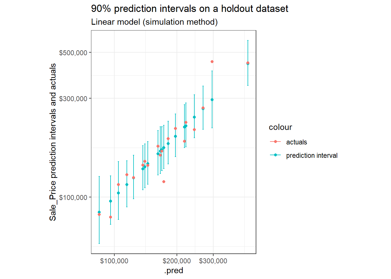

Simulation produced intervals show more differences in relative interval widths compared to those outputted with analytic methods (see Part 1, Review Prediction Intervals where the relative interval widths were nearly constant across predictions).

Interval Width

The relative widths of prediction intervals from the simulation based approach vary between observations by more than 10x what we saw in the Interval Widths using analytic methods¹³ (where interval width had a standard deviation of less than half a percentage point).

We also see greater differences in interval width between buckets of predictions (a range of about 5 to 6 percentage points vs 0.4).

This suggests the simulation based approach allows for greater differentiation in estimated levels of uncertainty by attributes¹⁴.

lm_sim_widths <- lm_sim_intervals %>% 
  mutate(interval_width = .pred_upper - .pred_lower,
         interval_pred_ratio = interval_width / .pred) %>% 
  mutate(price_grouped = ggplot2::cut_number(.pred, 5)) %>% 
  group_by(price_grouped) %>% 
  summarise(n = n(),
            mean_interval_width_percentage = mean(interval_pred_ratio),
            stdev = sd(interval_pred_ratio),
            stderror = sd(interval_pred_ratio) / sqrt(n)) %>% 
  mutate(x_tmp = str_sub(price_grouped, 2, -2)) %>% 
  separate(x_tmp, c("min", "max"), sep = ",") %>% 
  mutate(across(c(min, max), as.double)) %>% 
  select(-price_grouped) 

lm_sim_widths %>% 
  mutate(across(c(mean_interval_width_percentage, stdev, stderror), ~.x*100)) %>% 
  gt::gt() %>% 
  gt::fmt_number(c("stdev", "stderror"), decimals = 2) %>% 
  gt::fmt_number("mean_interval_width_percentage", decimals = 1)

n	mean_interval_width_percentage	stdev	stderror	min	max
147	55.7	8.44	0.70	43200	121000
146	51.0	4.97	0.41	121000	145000
146	50.2	2.84	0.23	145000	176000
146	50.7	5.07	0.42	176000	221000
146	51.8	8.02	0.66	221000	485000

Simultaneously, the average relative interval width is slightly more narrow: about 52% for the simulation based approach against 54% for the analytic method¹⁵.

lm_sim_intervals %>% 
  mutate(interval_width = .pred_upper - .pred_lower,
         interval_pred_ratio = interval_width / .pred) %>% 
  summarise(n = n(),
            mean_interval_width_percentage = mean(interval_pred_ratio),
            stderror = sd(interval_pred_ratio) / sqrt(n)) %>% 
  mutate(across(c(mean_interval_width_percentage, stderror), ~.x * 100)) %>% 
  gt::gt() %>% 
  gt::fmt_number(c("mean_interval_width_percentage", "stderror"), decimals = 2) %>% 
  gt::fmt_number("mean_interval_width_percentage", decimals = 1)

n	mean_interval_width_percentage	stderror
731	51.9	0.24

Coverage

Coverage is essentially the same: 92.2% (vs 92.7% for Coverage with the analytic method)¹⁶.

lm_sim_intervals %>%
  mutate(covered = ifelse(Sale_Price >= .pred_lower & Sale_Price <= .pred_upper, 1, 0)) %>% 
  summarise(n = n(),
            n_covered = sum(
              covered
            ),
            stderror = sd(covered) / sqrt(n),
            coverage_prop = n_covered / n) %>% 
  mutate(across(c(coverage_prop, stderror), ~.x * 100)) %>% 
  gt::gt() %>% 
  gt::fmt_number("stderror", decimals = 2) %>% 
  gt::fmt_number("coverage_prop", decimals = 1)

n	n_covered	stderror	coverage_prop
731	674	0.99	92.2

Coverage rates across quintiles:

lm_sim_intervals %>% 
  mutate(price_grouped = ggplot2::cut_number(.pred, 5)) %>% 
  mutate(covered = ifelse(Sale_Price >= .pred_lower & Sale_Price <= .pred_upper, 1, 0)) %>% 
  group_by(price_grouped) %>% 
  summarise(n = n(),
            n_covered = sum(
              covered
            ),
            stderror = sd(covered) / sqrt(n),
            n_prop = n_covered / n) %>% 
  mutate(x_tmp = str_sub(price_grouped, 2, -2)) %>% 
  separate(x_tmp, c("min", "max"), sep = ",") %>% 
  mutate(across(c(min, max), as.double)) %>% 
  ggplot(aes(x = forcats::fct_reorder(scales::dollar(max), max), y = n_prop))+
  geom_line(aes(group = 1))+
  geom_errorbar(aes(ymin = n_prop - 2 * stderror, ymax = n_prop + 2 * stderror))+
  coord_cartesian(ylim = c(0.70, 1.01))+
  # scale_x_discrete(guide = guide_axis(n.dodge = 2))+
  labs(x = "Max Predicted Price for Quintile",
       y = "Coverage at Quintile",
       title = "Coverage by Quintile of Predictions",
       subtitle = "On a holdout Set",
       caption = "Error bars represent {coverage} +/- 2 * {coverage standard error}")+
  theme_bw()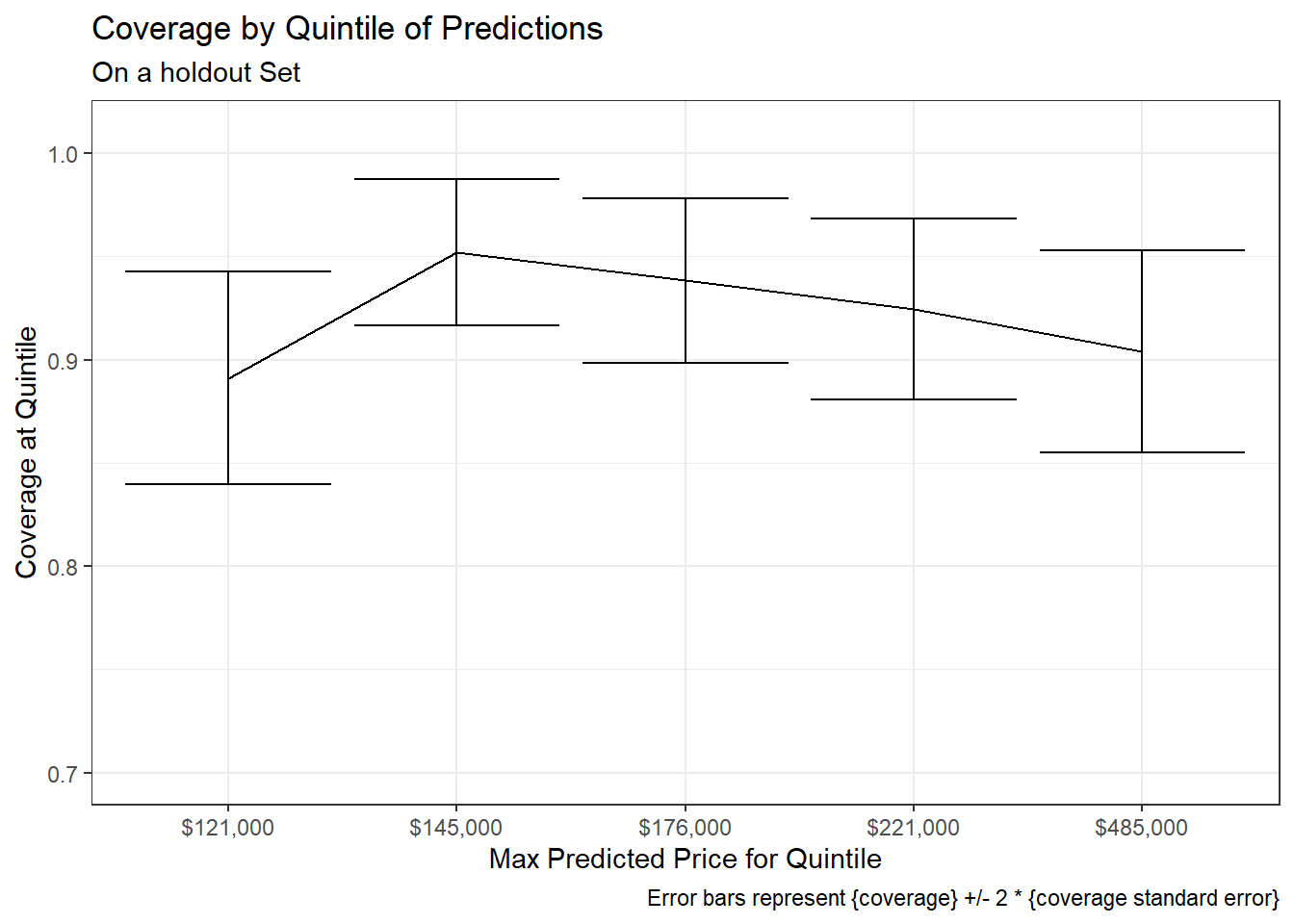

The overall pattern appears broadly similar to that seen in the analytic method. However coverage rates seem to be slightly more consistent across quintiles in the simulation based approach – an improvement over the analytic method (where coverage levels had appeared to be slightly more dependent upon quintile of predicted Sale_Price)¹⁷.

For example, a chi-squared test in the previous post had shown significant variation in coverage rates across quintiles when applied to the analytic method. However the same test applied to the results from the simulation based prediction intervals does not show a significant difference¹⁸.

lm_sim_intervals %>% 
  mutate(price_grouped = ggplot2::cut_number(.pred, 5)) %>% 
  mutate(covered = ifelse(Sale_Price >= .pred_lower & Sale_Price <= .pred_upper, 1, 0)) %>% 
  with(chisq.test(price_grouped, covered)) %>% 
  pander::pander()

Pearson’s Chi-squared test: `price_grouped` and `covered`
Test statistic	df	P value
4.987	4	0.2886

Keep in mind we are looking at just one model specification on one set of data¹⁹.

See Adjusting Procedure in the Appendix for a couple examples of circumstances where you might want to make changes to Procedure.

Closing Notes

This post walked through a rough implementation for simulating prediction intervals for arbitrary model types + preprocessing steps in a way that is loosely in the style of tidymodels. It represents a continuation on Understanding Prediction Intervals and is the second of three posts I am writing on prediction intervals. The third post will cover quantile regression.

Advantages of simulation based techniques for building prediction intervals:

can produce prediction intervals for model types that are intractable to produce estimates for analytically.
Even for model types that have analytic solutions for prediction intervals, simulation based approaches rely on fewer assumptions and can be more flexible²⁰.

Downsides:

These methods are far more computationally expensive as you will need to build a lot of models²¹.
- See Tidy Models with R, 10.4 for notes on how to set-up Parallel Processing.
For predictive inference, you still can’t drop all assumptions²².

Appendix

Conformal Inference

Highly related to what I presented in this post, the academic discipline of using out-of-sample data to create prediction intervals is known as conformal inference (much of the research in this field comes from Carnegie Mellon University and Royal Holloway University, London). I may do a follow-up post where I walk through a more formal example of using conformal inference. In the meantime, here are a few resources I glanced through²³:

ryantibs/conformal: github repo with conformalInference R package and links to relevant articles on distribution-free predictive inference. The way model types are specified by conformalInferene seems to be not too dissimilar from the approach I took in this post²⁴
donlnz/nonconformist: python package for conformal inference
Conformal Prediction: Link to Royal Holloway University website by creators of method – Vladimir Vovk and Alex Gammerman.
Assumption-free prediction intervals for black-box regression algorithms - Aaditya Ramdas (YouTube): professor at CMU giving overview of problem, approaches, and current “state-of-the-art”.
Tutorial on conformal inference, Dataiku article, Analytics Vidhya article

Other Examples Using Simulation

Here is a video walk-through of a simple example using a linear model:

A slightly modified version of this approach that adjusts for the leverage of the observations (leverage²⁵ has to do with distance of a point from the centroid of the data²⁶) can be found at this Cross Validated Thread.

Limitation with these examples (as encoded):

re-estimate some component of their prediction intervals based on performance on the data used to train the model.
are set-up for linear models

Confusion With Confidence Intervals

It seems to be common for people to seem to set-out to simulate prediction intervals but end-up simulating confidence intervals²⁷ – i.e. they account for uncertainty in estimating the model while forgetting to account for the uncertainty of the sample. I wrote more on this in Prediction Intervals and Confidence Intervals from Part 1²⁸.

Adjusting Procedure

Below are just a few examples. (Procedure is more just a toy set-up and by no means optimized.)

Coverage level depends on attribute(s)

If we see that coverage rates depend on predicted value of Sale_Price (or on some other attribute) we might:

try altering the pre-processing recipe
adjust Procedure to segment²⁹ the residuals by predicted Sale_Price and shuffle the errors within segments (rather than across the entire dataset). This would allow the uncertainty due to the sample to vary according to the predicted Sale_Price³⁰.

Random Splits Not Appropriate

The procedure I walk through assumes a random split in your data is fine and that your observations are iid. This is generally a requirement for using the bootstrap, however there are some approaches to using modified bootstrap that can adjust for this. In many cases it may make sense to have group or time based sampling schemes (see my presentation that discusses time-based resampling schemes). If a random sampling scheme is inappropriate, you will likely end-up creating too small of prediction intervals. I had considered making prep_interval() capable of taking in custom resampling specifications but did not set this up… but could be potentially edited.

Alternative Procedure With CV