In this post I will use incentives for sales representatives in pricing to provide examples of factors to consider when attempting to influence an existing distribution.
For instance, if you have a lever that pushes prices from low to high, using the lever to influence the prices adjacent to the right of the largest parts of the distribution will (likely, though contingent on a variety of factors) make the biggest impact on raising the average price attained. If the starting distribution is normal, this means incentives applied near the lower prices (the tail of the distribution) may have the smallest impact.
All figures in this post are created using the R programming language (see Rmarkdown document on github for code).
Simple Example
Imagine you have a product that can be sold anywhere from $100 to $150. Sales reps want to sell for as high of a price as possible and customers want to purchase for as low of a price as possible. In this tension your product ends-up selling, on average, for $125 and follows a truncated normal distribution with standard deviation of $101.
library(tidyverse)

theme_set(theme_bw())
data_distribution <- tibble(price = 100:150,
dens = dnorm(price, mean = 125, sd = 10)) %>%
mutate(dens_scaled = dens / sum(dens))
data_distribution %>%
ggplot(aes(x = price, y = dens_scaled))+
geom_col()+
ylim(c(0, 0.15))+
labs(y = "density")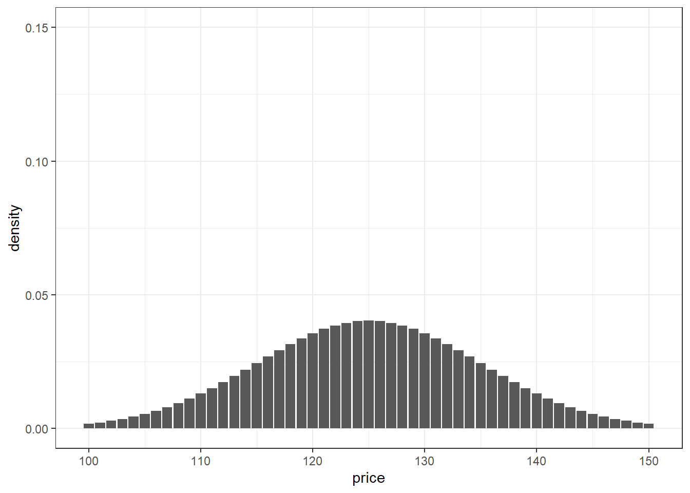
Applying Incentives
Executive leadership wants to apply additional incentives on sales reps to keep prices high2. They task you with setting-up a tiered compensation scheme whereby deals at the top-end of the distribution get a higher compensation rate compared to deals at the bottom end of the distribution.
Applying such an additional incentive on sales teams has the potential advantage of pushing some proportion of deals to a higher price3. There are also Trade-offs associated with such an initiative (indicated in the Appendix), these will be ignored for the purposes of this exercise.
Say you decide to set cut-points to split the distribution into quartiles such that sales reps get larger bonuses if their deals fall into higher quartiles.
data_distribution %>%
  mutate(cum_dens = cumsum(dens_scaled),
         quartile = (cum_dens) %/% 0.2500001 + 1,
         quartile = as.factor(quartile)) %>%
  rename(initial_quartile = quartile) %>%
  ggplot(aes(x = price, y = dens_scaled, fill = initial_quartile))+
  geom_col()+
  scale_fill_discrete(type = c("deeppink", "orange", "yellow2", "royalblue"))+
  ylim(c(0, 0.15))+
  labs(y = "density")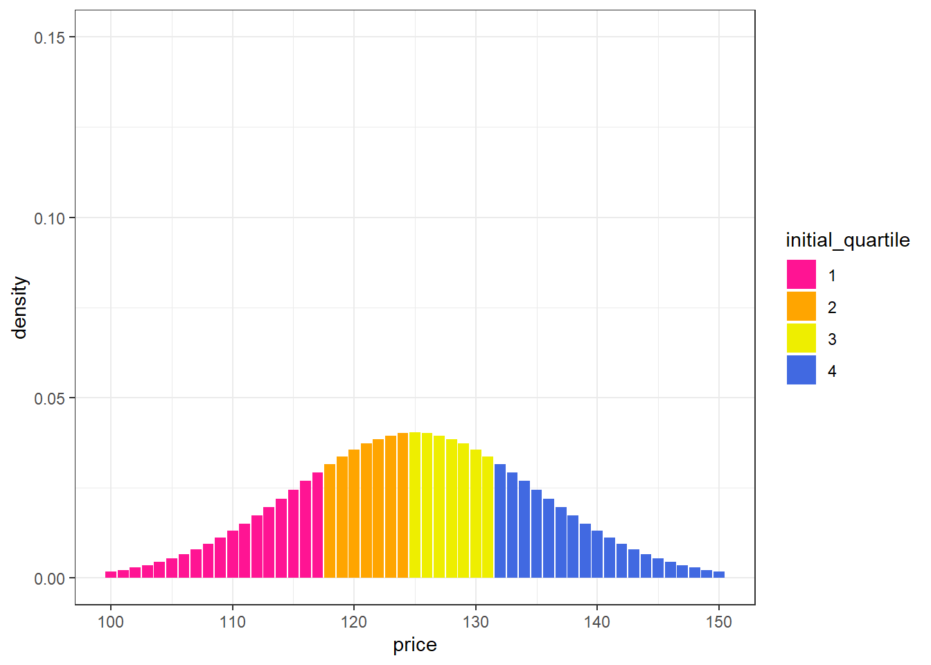
Applying incentives is likely to lead to a different distribution for future deals.
- Consider what the relevant factors and assumptions are in influencing the existing distribution.
- Take a moment to hypothesize what the new distribution will look like after incentives are applied.
After applying incentives the resulting distribution is likely to depend on:
- The starting distribution4 of deals.
- What the incentives are and how they influence the initial distribution.
- How this influence degrades the farther away the starting position of a deal is from the next tier up in incentives.
You could paramaterize this problem and model the expected distribution. Making some Simple Assumptions (described in the Appendix), the chart below shows a (potential) resulting distribution after applying the incentives.
data_distribution <- data_distribution %>%
  mutate(cum_dens = cumsum(dens_scaled),
         incentive = ((cum_dens) %/% 0.2500001) * 5,
         incentive_delta = ifelse(incentive == 15, 0, 5)) # hard coded
# very inefficient approach computationally
get_row_bump <- function(price_current){
current_incentive <- data_distribution %>%
filter(price == {{price_current}}) %>%
pull(incentive)
output <- data_distribution %>%
filter(price > {{price_current}}, incentive > current_incentive) %>%
head(1) %>%
pull(price)
if(length(output) == 0) output <- NA
output
}
proportion_raised <- function(density, incentive_delta, distance){
decay <- 0.75^(distance - 1)
incentive <- incentive_delta * 0.15
# incentive <- ifelse(incentive > 1, 1, incentive)
density * decay * incentive
}data_distribution %>%
mutate(quartile = (cum_dens) %/% 0.2500001 + 1,
quartile = as.factor(quartile)) %>%
mutate(price_next = map_int(price, get_row_bump),
price_dist = price_next - price) %>%
mutate(density_convert = proportion_raised(dens_scaled, incentive_delta, price_dist)) %>%
select(-dens) %>%
# add converted density to nearest point
group_by(incentive) %>%
mutate(dens_convert_total = sum(density_convert),
price_switch = price == min(price)) %>%
ungroup() %>%
mutate(dens_convert_total = lag(dens_convert_total),
dens_convert_total = ifelse(price_switch, dens_convert_total, 0)) %>%
# na's to 0's
mutate(across(c(density_convert, dens_convert_total), ~ifelse(is.na(.x), 0, .x))) %>%
# adjust percentages
mutate(dens_adj = dens_scaled - density_convert + dens_convert_total) %>%
rename(initial_quartile = quartile) %>%
# graph
ggplot(aes(x = price))+
geom_col(aes(y = dens_adj, fill = initial_quartile))+
scale_fill_discrete(type = c("deeppink", "orange", "yellow2", "royalblue"))+
ylim(c(0, 0.15))+
labs(y = "density")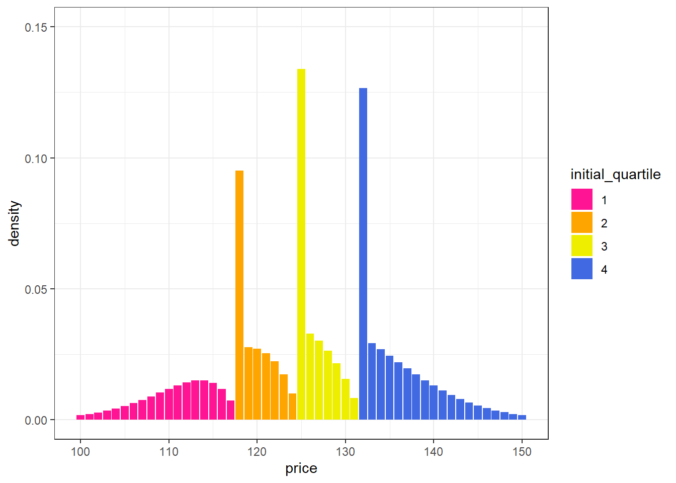
Gray bars in the chart below indicate where (on the original distribution) movement to a higher tier will occur.
data_distribution %>%
  mutate(quartile = (cum_dens) %/% 0.2500001 + 1,
         quartile = as.factor(quartile)) %>%
  mutate(price_next = map_int(price, get_row_bump),
         price_dist = price_next - price) %>%
  mutate(density_convert = proportion_raised(dens_scaled, incentive_delta, price_dist)) %>%
  select(-dens) %>%
  rename(initial_quartile = quartile) %>%
  ggplot(aes(x = price))+
  geom_col(aes(y = dens_scaled, fill = initial_quartile))+
  geom_col(aes(y = density_convert), fill = "gray")+
  scale_fill_discrete(type = c("deeppink", "orange", "yellow2", "royalblue"))+
  ylim(c(0, 0.15))+
  labs(y = "density")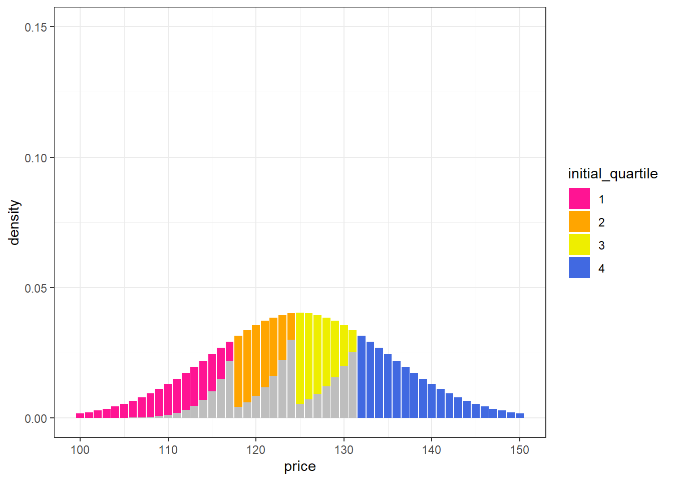
Takeaways of Resulting Distribution
The greatest proportion of deals were moved from orange to yellow and from yellow to blue. Pink to orange had the least amount of movement (due to the first quartile being spread across a wider range).
data_distribution %>%
  mutate(quartile = (cum_dens) %/% 0.2500001 + 1,
         quartile = as.factor(quartile)) %>%
  mutate(price_next = map_int(price, get_row_bump),
         price_dist = price_next - price) %>%
  mutate(density_convert = proportion_raised(dens_scaled, incentive_delta, price_dist)) %>%
  select(-dens) %>%
  mutate(incentive = case_when(incentive == 0 ~ "pink to orange",
                               incentive == 5 ~ "orange to yellow",
                               incentive == 10 ~ "yellow to blue",
                               TRUE ~ "stayed blue") %>% fct_inorder()) %>%
  group_by(incentive) %>%
  summarise(density_converted = sum(density_convert) %>% round(3)) %>%
knitr::kable()| incentive | density_converted |
|---|---|
| pink to orange | 0.068 |
| orange to yellow | 0.099 |
| yellow to blue | 0.095 |
| stayed blue | NA |
Incentives Make the Biggest Difference When Nearer to the Largest Parts of the Distribution Susceptible to Change
Because these incentives slide deals from lower prices to higher prices, those cut-points that are just above the most dense parts of the distribution have the biggest impacts on the post-incentivized distribution. For a normal distribution, such as this one, that means incentives just to the right of the first quartile have the smallest impact. (Importantly, this assumes susceptibility to rightward mobility is evenly distributed across the starting distribution.)
How Many Thresholds
For many reasonable assumptions5, having more thresholds will lead to greater movement upwards in the distribution. Similarly, a continuous application of incentives (i.e. sales reps get higher compensation for every point they move up on the distribution) can be optimal under certain assumptions as well6.
Quartiles change
After applying the incentives, the cut-points for segmenting the distribution into quartiles on future deals will be different. Given your assumptions, you could try forecasting where the new quartiles will exist (after applying the incentives) and adjust the bonus thresholds proactively.
Thresholds for incentives could also be adjusted dynamically. For example based on a rolling average of the quartiles of recent deals. In this approach, you apply initial incentives and then allow them to change dynamically depending on the resulting distribution of deals – setting guard rails where appropriate. An advantage to this dynamic approach is that the compensation rates gets set based on behavior7 – which is helpful in cases where you may not trust your ability to set appropriate thresholds.
Think Carefully About Assumptions
Simulating the expected outcome based on assumptions such as the ones described in this post are helpful in thoughtfully elucidating the problem for yourself or for others. Assumptions do not need to be perfect to be useful for thinking through the problem but they should lean towards the actual patterns in your example.
How do Incentives Aggregate?
In this case, we are assuming incentives aggregate in a linear way. This means that five 1 ppt incentives have the same amount of influence as one 5 ppt incentive. It could be that the former is more influential (people prefer many small bonuses) or the latter is more influential (people prefer one large bonuses)8.
It could also be that there is a ‘correct’ size of incentive and that too small an incentive makes no difference but a large incentive has diminishing returns. If this is the case a logistic function or other ‘S’ shaped function may be more reasonable for modeling the influence of incentives.
How does Influence Degrade With Distance From Incentives?
In this case, we are assuming the influence of an incentive exponential decays (the influence decreases by 25% for every point we move from the cut-point). Hence being only a few points away from a cut-point has a big impact, but the degradation is less with each point we move away.
How is Slack Distributed
I assumed slack (i.e. the possibility of deals being influenced by incentives) was equally distributed. (It could be that slack is distributed disproportionally towards the lower ends of the distribution for example.)
How to Set Assumptions
- Start with what makes sense (e.g. normal distributions are often good starting places)
- Review historical data
- Set-up formal tests (e.g. create hypotheses and see how behavior adjusts as you change incentives on random subsets of your sales representatives)
Appendix
Simple Assumptions
For this example, we will say the incentives you established are higher compensation rates depending on which quartile the deal falls in. If the deal falls in the lowest quartile they get no increase, in the 2nd quartile they get a 5 percentage point (ppt) increase in pay, the 3rd a 10 ppt increase, the 4th a 15 ppt increase9.
For now I’ll pick some overly simple but sensible values for each question:
As indicated, we are assuming the ‘natural’ distribution of prices is roughly normal
We will assume that for every 1 ppt change in incentive that 15% of the deals immediately to the right of the cut-off will be moved up to the cut-off value.
We will assume that this influence degrades by 25% for every dollar you move from the cut-point10. I am ignoring the possibility of deals jumping more than on level (e.g. deals moving from the 1st quartile to the 3rd quartile)11.
Trade-offs
- A sales rep may have been able to sell more product at a lower price.
- The additional incentive causes some deals (those selling for lower prices) to be passed on because the incentive to close on the deal for reps has been lowered (this may be intentional in that the impact on price erosion of these deals is worth the decrease in sales…).
- You may have to pay your sales reps more
- Applying such incentives may create additional bureaucratic hurdles in closing deals that increase the friction of closing deals, causing some percentage of deals to be lost
- It could be that deals don’t have slack in them and are already optimal…
- Any change in pricing behavior has the risk of upsetting customers or having downstream affects.
Ideally the organization is able to take into account risks and advantages in pricing and set-up incentives that are focused on overall profitability and firm growth (not just in terms of a single factor).
Limits for Y axis appear too large for this chart but are set from 0 to 0.15 so as to be consistent with similar figures later in post.↩︎
E.g. to prevent brand erosion, improve margins, etc.↩︎
This assumes that there is some slack in the existing deals and that representatives are in a position to impact this and will do so if provided higher incentives.↩︎
or potentially a ‘natural’ distribution that would exist in the absence of incentives↩︎
Key to this assumption is how incentives degrade as you move farther from a cut-point.↩︎
These do not consider potential psychological impacts or difficulty of implementation.↩︎
Similar to in a market.↩︎
Research into psychological biases suggests the former may be true.↩︎
You could also construct this such that lower quartiles have negative incentives and higher quartiles have positive incentives.↩︎
The functions governing these behaviors are almost certainly more sophisticated.↩︎
Factoring this possibility in would likely lead to incentives at the higher quartiles making a slightly larger impact.↩︎