Say you want to map an operation or list of operations across all two-way1 combinations of a set of variables/columns in a dataframe. For example, you may be doing feature engineering and want to create a set of interaction terms, ratios, etc2. You may be interested in computing a summary statistic across all pairwise combinations of a given set of variables3. In some cases there may be a pairwise implementation already available, e.g. R’s cor() function for computing correlations4. In other cases one may not exist or is not easy to use5. In this post I’ll walk through an example6 explaining code and steps for setting-up arbitrary pairwise operations across sets of variables.
I’ll break my approach down into several steps:
I. Nest and pivot
II. Expand combinations
III. Filter redundancies
IV. Map function(s)
V. Return to normal dataframe
VI. Bind back to data
If your interest is only in computing summary statistics (as opposed to modifying an existing dataframe with new columns / features),then only steps I - IV are needed.
Relevant software and style:
I will primarily be using R’s tidyverse packages. I make frequent use of lists as columns within dataframes – if you are new to these, see my previous talk and the resources7 I link to in the description.
Throughout this post, wherever I write “dataframe” I really mean “tibble” (a dataframe with minor changes to default options and printing behavior). Also note that I am using dplyr 0.8.3 rather than the newly released 1.0.08.
library(tidyverse)Data
I’ll use the ames housing dataset across examples.
ames <- AmesHousing::make_ames()Specifically, I’ll focus on ten numeric columns that, based on a random sample of 1000 rows, show the highest correlation with Sale_Price9.
set.seed(2020)
ames_cols <- ames %>%
  select_if(is.numeric) %>%
  sample_n(1000) %>%
  corrr::correlate() %>%
  corrr::focus(Sale_Price) %>%
  arrange(-abs(Sale_Price)) %>%
  head(10) %>%
  pull(rowname)

ames_subset <- select(ames, ames_cols) %>%
  # Could normalize data or do other prep
  # but is not pertinent for examples
  mutate_all(as.double)
Overview
I. Nest and pivot
There are a variety of ways to make lists into columns within a dataframe. In the example below, I first use summarise_all(.tbl = ames_subset, .funs = list) to create a one row dataframe where each column is a list containing a single element and each individual element corresponds with a numeric vector of length 2930.
After nesting, I pivot10 the columns leaving a dataframe with two columns:
varthe variable namesvectora list where each element contains the associated vector
df_lists <- ames_subset %>%
  summarise_all(list) %>%
  pivot_longer(cols = everything(),
               names_to = "var",
               values_to = "vector") %>%
  print()
## # A tibble: 10 x 2
## var vector
## <chr> <list>
## 1 Gr_Liv_Area <dbl [2,930]>
## 2 Garage_Cars <dbl [2,930]>
## 3 Garage_Area <dbl [2,930]>
## 4 Total_Bsmt_SF <dbl [2,930]>
## 5 First_Flr_SF <dbl [2,930]>
## 6 Year_Built <dbl [2,930]>
## 7 Full_Bath <dbl [2,930]>
## 8 Year_Remod_Add <dbl [2,930]>
## 9 TotRms_AbvGrd <dbl [2,930]>
## 10 Fireplaces <dbl [2,930]>See Pivot and then summarise for a nearly identical approach with just an altered order of steps. Also see Nested tibbles for how you could create a list-column of dataframes11 rather than vectors.
What if my variables are across rows not columns?
For example, pretend you want to see if Sale_Price is different across Mo_Sold. Perhaps you started by doing an F-test, found that to be significant, and now want to do pairwise t-tests across the samples of Sale_Price for each Mo_Sold. To set this up, you will want a group_by() rather than a pivot_longer() step. E.g.
ames %>%
  group_by(Mo_Sold) %>%
  summarise(Sale_Price = list(Sale_Price))
## # A tibble: 12 x 2
## Mo_Sold Sale_Price
## <int> <list>
## 1 1 <int [123]>
## 2 2 <int [133]>
## 3 3 <int [232]>
## 4 4 <int [279]>
## 5 5 <int [395]>
## 6 6 <int [505]>
## 7 7 <int [449]>
## 8 8 <int [233]>
## 9 9 <int [161]>
## 10 10 <int [173]>
## 11 11 <int [143]>
## 12 12 <int [104]>At which point your data is in fundamentally the same form as was created in the previous code chunk (at least for if we only care about computing summary metrics that don’t require vectors of equal length12) so you can move onto II. Expand combinations.
If the variables needed for your combinations of interest are across both rows and columns, you may want to use both pivot_longer() and group_by() steps and may need to make a few small modifications.
II. Expand combinations
I then use tidyr::nesting() within tidyr::expand() to make all 2-way combinations of our rows.
df_lists_comb <- expand(df_lists,
                        nesting(var, vector),
                        nesting(var2 = var, vector2 = vector)) %>%
  print()
## # A tibble: 100 x 4
## var vector var2 vector2
## <chr> <list> <chr> <list>
## 1 Fireplaces <dbl [2,930]> Fireplaces <dbl [2,930]>
## 2 Fireplaces <dbl [2,930]> First_Flr_SF <dbl [2,930]>
## 3 Fireplaces <dbl [2,930]> Full_Bath <dbl [2,930]>
## 4 Fireplaces <dbl [2,930]> Garage_Area <dbl [2,930]>
## 5 Fireplaces <dbl [2,930]> Garage_Cars <dbl [2,930]>
## 6 Fireplaces <dbl [2,930]> Gr_Liv_Area <dbl [2,930]>
## 7 Fireplaces <dbl [2,930]> Total_Bsmt_SF <dbl [2,930]>
## 8 Fireplaces <dbl [2,930]> TotRms_AbvGrd <dbl [2,930]>
## 9 Fireplaces <dbl [2,930]> Year_Built <dbl [2,930]>
## 10 Fireplaces <dbl [2,930]> Year_Remod_Add <dbl [2,930]>
## # ... with 90 more rowsSee Expand via join for an alternative approach using the dplyr::*_join() operations.
You could make a strong case that this step should be after III. Filter redundancies13. However putting it beforehand makes the required code easier to write and to read.
III. Filter redundancies
Filter-out redundant columns, sort the rows, better organize the columns.
df_lists_comb <- df_lists_comb %>%
  filter(!(var == var2)) %>%
  arrange(var, var2) %>%
  mutate(vars = paste0(var, ".", var2)) %>%
  select(contains("var"), everything()) %>%
  print()
## # A tibble: 90 x 5
## var var2 vars vector vector2
## <chr> <chr> <chr> <list> <list>
## 1 Fireplaces First_Flr_SF Fireplaces.First_Flr_~ <dbl [2,93~ <dbl [2,93~
## 2 Fireplaces Full_Bath Fireplaces.Full_Bath <dbl [2,93~ <dbl [2,93~
## 3 Fireplaces Garage_Area Fireplaces.Garage_Area <dbl [2,93~ <dbl [2,93~
## 4 Fireplaces Garage_Cars Fireplaces.Garage_Cars <dbl [2,93~ <dbl [2,93~
## 5 Fireplaces Gr_Liv_Area Fireplaces.Gr_Liv_Area <dbl [2,93~ <dbl [2,93~
## 6 Fireplaces Total_Bsmt_SF Fireplaces.Total_Bsmt~ <dbl [2,93~ <dbl [2,93~
## 7 Fireplaces TotRms_AbvGrd Fireplaces.TotRms_Abv~ <dbl [2,93~ <dbl [2,93~
## 8 Fireplaces Year_Built Fireplaces.Year_Built <dbl [2,93~ <dbl [2,93~
## 9 Fireplaces Year_Remod_A~ Fireplaces.Year_Remod~ <dbl [2,93~ <dbl [2,93~
## 10 First_Flr_~ Fireplaces First_Flr_SF.Fireplac~ <dbl [2,93~ <dbl [2,93~
## # ... with 80 more rowsIf your operation of interest is associative14, apply a filter to remove additional redundant combinations.
c_sort_collapse <- function(...){
  c(...) %>%
    sort() %>%
    str_c(collapse = ".")
}

df_lists_comb_as <- df_lists_comb %>%
  mutate(vars = map2_chr(.x = var,
                         .y = var2,
                         .f = c_sort_collapse)) %>%
  distinct(vars, .keep_all = TRUE)
IV. Map function(s)
Each row of your dataframe now contains the relevant combinations of variables and is ready to have any arbitrary function(s) mapped across them.
Example with summary statistic15:
For example, let’s say we want to compute the p-value of the correlation coefficient for each pair16.
pairs_cor_pvalues <- df_lists_comb_as %>%
  mutate(cor_pvalue = map2(vector, vector2, cor.test) %>% map_dbl("p.value"),
         vars = fct_reorder(vars, -cor_pvalue)) %>%
  arrange(cor_pvalue) %>%
  print()
## # A tibble: 45 x 6
## var var2 vars vector vector2 cor_pvalue
## <chr> <chr> <fct> <list> <list> <dbl>
## 1 First_Flr~ Total_Bsm~ First_Flr_SF.Tot~ <dbl [2,9~ <dbl [2,9~ 0.
## 2 Full_Bath Gr_Liv_Ar~ Full_Bath.Gr_Liv~ <dbl [2,9~ <dbl [2,9~ 0.
## 3 Garage_Ar~ Garage_Ca~ Garage_Area.Gara~ <dbl [2,9~ <dbl [2,9~ 0.
## 4 Gr_Liv_Ar~ TotRms_Ab~ Gr_Liv_Area.TotR~ <dbl [2,9~ <dbl [2,9~ 0.
## 5 Year_Built Year_Remo~ Year_Built.Year_~ <dbl [2,9~ <dbl [2,9~ 7.85e-301
## 6 First_Flr~ Gr_Liv_Ar~ First_Flr_SF.Gr_~ <dbl [2,9~ <dbl [2,9~ 8.17e-244
## 7 Garage_Ca~ Year_Built Garage_Cars.Year~ <dbl [2,9~ <dbl [2,9~ 1.57e-219
## 8 Full_Bath TotRms_Ab~ Full_Bath.TotRms~ <dbl [2,9~ <dbl [2,9~ 1.24e-210
## 9 First_Flr~ Garage_Ar~ First_Flr_SF.Gar~ <dbl [2,9~ <dbl [2,9~ 8.16e-178
## 10 Garage_Ca~ Gr_Liv_Ar~ Garage_Cars.Gr_L~ <dbl [2,9~ <dbl [2,9~ 4.80e-175
## # ... with 35 more rowsFor fun, let’s plot the most significant associations onto a bar graph.
pairs_cor_pvalues %>%
  head(15) %>%
  mutate(cor_pvalue_nlog = -log(cor_pvalue)) %>%
  ggplot(aes(x = vars,
             y = cor_pvalue_nlog,
             fill = is.infinite(cor_pvalue_nlog) %>% factor(c(T, F))))+
  geom_col()+
  coord_flip()+
  theme_bw()+
  labs(title = "We are confident that garage area and # of garage cars are correlated",
       y = "Negative log of p-value of correlation coefficient",
       x = "Variable combinations",
       fill = "Too high to\nmeaningfully\ndifferentiate:")+
  theme(plot.title.position = "plot")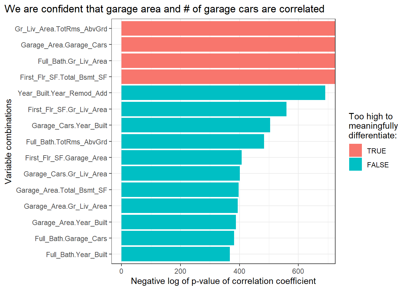
You could use this approach to calculate any pairwise summary statistic. For example, see gist where I calculate the K-S statistic across each combination of a group of distributions.
If you only care about computing summary statistics on your pairwise combinations, (and not adding new columns onto your original dataframe) you can stop here.
Example with transformations17:
Back to the feature engineering example, perhaps we want to create new features of the difference and quotient of each combination of our variables.
new_features_prep1 <- df_lists_comb %>%
  mutate(difference = map2(vector, vector2, `-`),
         ratio = map2(vector, vector2, `/`))
V. Return to normal dataframe
The next set of steps will put our data back into a more traditional form consistent with our starting dataframe/tibble.
First let’s revert our data to a form similar to where it was at the end of I. Nest and pivot where we had two columns:
- one with our variable names
- a second containing a list-column of vectors
new_features_prep2 <- new_features_prep1 %>%
  pivot_longer(cols = c(difference, ratio)) %>% # 1
  mutate(name_vars = str_c(var, name, var2, sep = ".")) %>% # 2
  select(name_vars, value) # 3
At the end of each line of code above is a number corresponding with the following explanations:
- if we had done just one operation, this step would not be needed, but we did multiple operations, created multiple list-columns (
differenceandratio) which we need to get into a single list-column - create new variable name that combines constituent variable names with name of transformation
- remove old columns
Next we simply apply the inverse of those operations performed in I. Nest and pivot.
new_features <- new_features_prep2 %>%
  pivot_wider(values_from = value,
              names_from = name_vars) %>%
  unnest(cols = everything())
The new features will add a good number of columns onto our original dataset18.
dim(new_features)## [1] 2930 180VI. Bind back to data
I then bind the new features back onto the original subsetted dataframe.
ames_data_features <- bind_cols(ames_subset, new_features)At which point I could do further exploring, feature engineering, model building, etc.
Functionalize
I put these steps into a few (unpolished) functions found at this gist19.
devtools::source_gist("https://gist.github.com/brshallo/f92a5820030e21cfed8f823a6e1d56e1")operations_combinations() takes in your dataframe, the set of numeric columns to create pairwise combinations from, and a list of functions20 to apply.
Example creating & evaluating features
Let’s use the new operations_combinations() function to create new columns for the differences and quotients between all pairwise combinations of our variables of interest.
ames_data_features_example <- operations_combinations(
  df = mutate_if(ames, is.numeric, as.double),
  one_of(ames_cols),
  funs = list("/", "-"),
  funs_names = list("ratio", "difference"),
  associative = FALSE
)
Perhaps you want to calculate some measure of association between your features and a target of interest. To keep things simple, I’ll remove any columns that contain any NA’s or infinite values.
features_keep <- ames_data_features_example %>%
  keep(is.numeric) %>%
  keep(~sum(is.na(.) | is.infinite(.)) == 0) %>%
  colnames()
Maybe, for some reason, you want to see the statistical significance of the correlation of each feature with Sale_Price when weighting by Lot_Area. I’ll calculate these across variables (and a random sample of 1500 observations) then plot them on a histogram.
set.seed(1234)
ames_data_features_example %>%
  sample_n(1500) %>%
  summarise_at(
    .vars = features_keep[!(features_keep %in% c("Sale_Price", "Lot_Area"))],
    .funs = ~weights::wtd.cor(., Sale_Price, weight = Lot_Area)[1]) %>%
  gather() %>% # gather() is an older version of pivot_longer() w/ fewer parameters
  ggplot(aes(x = value))+
  geom_vline(xintercept = 0, colour = "lightgray", size = 2)+
  geom_histogram()+
  scale_x_continuous(labels = scales::comma)+
  labs(title = "Distribution of correlations with Sale_Price",
       subtitle = "Weighted by Lot Area",
       x = "Weighted correlation coefficient")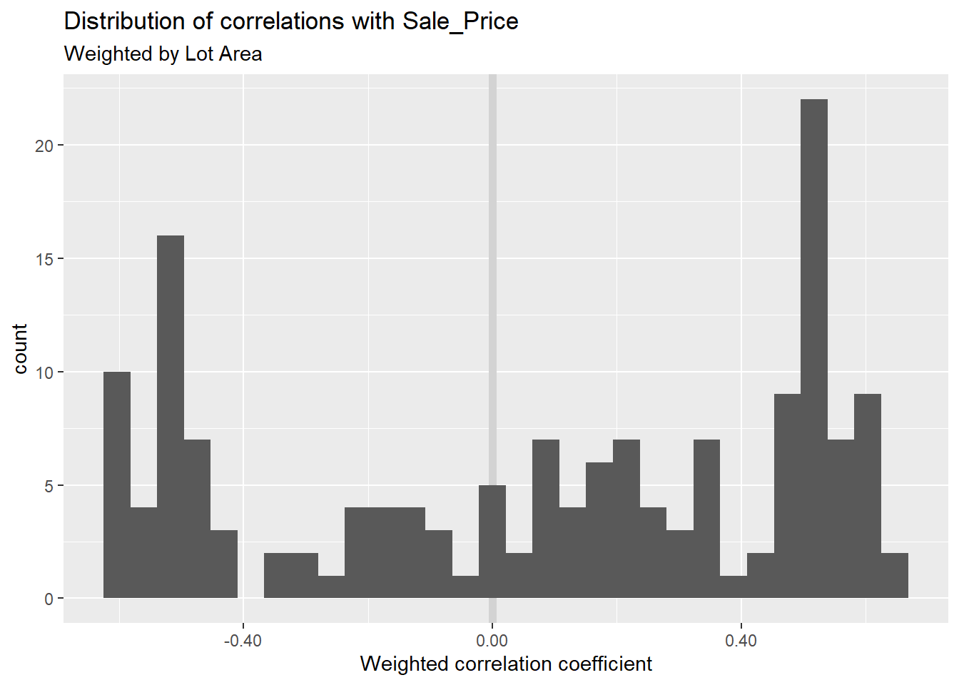
If doing predictive modeling or inference you may want to fit any transformations and analysis into a tidymodels pipeline or other framework. For some brief notes on this see Interactions example, tidymodels.
When is this approach inappropriate?
Combinatorial growth is very fast21. As you increase either the number of variables in your pool or the size of each set, you will quickly bump into computational limitations.
Tidyverse packages are optimized to be efficient. However operations with matrices or other specialized formats22 are generally faster23 than with dataframes/tibbles. If you are running into computational challenges but prefer to stick with a tidyverse aesthetic (which uses dataframes as a cornerstone), you might:
- Use heuristics to reduce the number of variables or operations you need to perform (e.g. take a sample, use a preliminary filter, a step-wise like iteration, etc.)
- Look for packages that abstract the storage and computationally heavy operations away24 and then return back an output in a convenient form25
- Improve the efficiency of your code (e.g. filter redundancies before rather than after expanding combinations)26
- Consider parralelizing
- Use matrices27
For example, you could use an approach like the one I walk through to calculate pairwise correlations between each of your variables. However, the cor() function would do this much more efficiently if called on a matrix or traditional dataframe structure (or you could also use the corrr package within the tidymodels suite which calls cor() in the back-end28).
However, for many operations…
- there may not be an efficient pairwise implementation available / accessible
- the slower computation may not matter or can be mitigated in some way
These situations29 are where the approach I walked through is most appropriate.
Appendix
Interactions example, tidymodels
A good example for creating and evaluating interaction terms30 is in The Brute-Force Approach to Identifying Predictive Interactions, Simple Screening section of Max Kuhn and Kjell Johnson’s (free) online book “Feature Engineering and Selection: A Practical Approach for Predictive Models”.
The source code shows another approach for combining variables. The author uses…
combn()to create all combinations of variable names which are then…- turned into formulas and passed into
recipes::step_interact(), specifying the new columns to be created31… - for each interaction term…
- in each associated model being evaluated
The example uses a mix of packages and styles and is not a purely tidy approach – tidymodels has also gone through a lot of development since “Feature Engineering and Selection…” was published in 201932. Section 11.2 on Greedy Search Methods, Simple Filters is also highly relevant.
Expand via join
You can take advantage of join33 behavior to create all possible row combinations. In this case, the output will be the same as shown when using expand() (except row order will be different).
left_join(mutate(df_lists, id = 1),
          mutate(df_lists, id = 1) %>% rename_at(vars(-one_of("id")), paste0, "2")) %>%
  select(-id)
Nested tibbles
Creates list of tibbles rather than list of vectors – typically the first way lists as columns in dataframes is introduced.
ames_subset %>%
  pivot_longer(everything(), names_to = "var", values_to = "list") %>%
  group_by(var) %>%
  nest()
Pivot and then summarise
(Almost) equivalent to the example in I. Nest and pivot. Steps just run in a different order (row order will also be different).
ames_test %>%
  pivot_longer(cols = everything(),
             names_to = "var",
             values_to = "vector") %>%
  group_by(var) %>%
  summarise_all(list)
Session info
sessionInfo()## R version 3.5.1 (2018-07-02)
## Platform: x86_64-w64-mingw32/x64 (64-bit)
## Running under: Windows 10 x64 (build 18362)
##
## Matrix products: default
##
## locale:
## [1] LC_COLLATE=English_United States.1252
## [2] LC_CTYPE=English_United States.1252
## [3] LC_MONETARY=English_United States.1252
## [4] LC_NUMERIC=C
## [5] LC_TIME=English_United States.1252
##
## attached base packages:
## [1] stats graphics grDevices utils datasets methods base
##
## other attached packages:
## [1] forcats_0.4.0 stringr_1.4.0 dplyr_0.8.3 purrr_0.3.3
## [5] readr_1.3.1 tidyr_1.0.0 tibble_2.1.3 ggplot2_3.3.0
## [9] tidyverse_1.2.1
##
## loaded via a namespace (and not attached):
## [1] nlme_3.1-137 fs_1.3.2 usethis_1.4.0
## [4] lubridate_1.7.4 devtools_2.0.0 RColorBrewer_1.1-2
## [7] progress_1.2.2 httr_1.4.0 rprojroot_1.3-2
## [10] tools_3.5.1 backports_1.1.5 utf8_1.1.4
## [13] R6_2.4.1 rpart_4.1-13 Hmisc_4.1-1
## [16] colorspace_1.4-1 nnet_7.3-12 withr_2.1.2
## [19] gridExtra_2.3 tidyselect_0.2.5 prettyunits_1.0.2
## [22] processx_3.3.1 curl_3.3 compiler_3.5.1
## [25] cli_1.9.9.9000 rvest_0.3.4 htmlTable_1.12
## [28] mice_3.8.0 xml2_1.2.0 desc_1.2.0
## [31] labeling_0.3 bookdown_0.11 checkmate_1.8.5
## [34] scales_1.1.0 corrr_0.4.2 callr_3.2.0
## [37] digest_0.6.25 foreign_0.8-70 rmarkdown_1.13
## [40] base64enc_0.1-3 pkgconfig_2.0.3 htmltools_0.3.6
## [43] sessioninfo_1.1.1 htmlwidgets_1.3 rlang_0.4.5
## [46] readxl_1.3.1 rstudioapi_0.10 farver_2.0.1
## [49] generics_0.0.2 jsonlite_1.6.1 gtools_3.8.1
## [52] acepack_1.4.1 magrittr_1.5 Formula_1.2-3
## [55] Matrix_1.2-14 Rcpp_1.0.4 munsell_0.5.0
## [58] fansi_0.4.0 lifecycle_0.1.0 weights_1.0.1
## [61] stringi_1.4.6 yaml_2.2.0 pkgbuild_1.0.2
## [64] grid_3.5.1 gdata_2.18.0 crayon_1.3.4
## [67] lattice_0.20-35 haven_2.1.0 splines_3.5.1
## [70] hms_0.5.2 knitr_1.23 ps_1.3.0
## [73] pillar_1.4.2 pkgload_1.0.2 glue_1.3.1
## [76] evaluate_0.14 blogdown_0.15 latticeExtra_0.6-28
## [79] data.table_1.12.8 remotes_2.1.0 modelr_0.1.4
## [82] vctrs_0.2.4 testthat_2.0.0 cellranger_1.1.0
## [85] gtable_0.3.0 assertthat_0.2.1 xfun_0.8
## [88] broom_0.5.2 AmesHousing_0.0.3 survival_2.42-3
## [91] memoise_1.1.0 cluster_2.0.7-1 ellipsis_0.3.0Will focus on two-way example in this post, but could use similar methods to make more generalizable solution across n-way examples. If I were to do this, the code below would change. E.g.
- to use
pmap*()operations overmap2*()operations - I’d need to make some functions that make it so I can remove all the places where I have
varandvar2type column names hard-coded - Alternatively, I might shift approaches and make better use of
combn()
- to use
Though this “throw everything and the kitchen-sink” approach may not always be a good idea.↩
I’ve done this type of operation in a variety of ways. Sometimes without any really good reason as to why I used one approach or another. It isn’t completely clear (at least to me) the recommended way of doing these type of operations within the tidyverse – hence the diversity of my approaches in the past and deciding to document the typical steps in the approach I take… via writing this post.↩
Or the tidymodels implementation
corrr::correlate()in the corrr package.↩or is not in a style you prefer↩
I’ll also reference related approaches / small tweaks (putting those materials in the Appendix. This is by no means an exhaustive list (e.g. don’t have an example with a
forloop or with a%do%operator). The source code of my post on Ambiguous Absolute Value signs shows a related but more complex / messy approach on a combinatorics problem.↩In particular, the chapters on “Iteration” and “Many Models” in R for Data Science. I would also recommend Rebecca Barter’s Learn to purrr blog post.↩
The new
dplyr1.0.0. contains new functions that would have been potentially useful for several of these operations. I highly recommend checking these updates out in the various recent posts by Hadley Wickham. Some of the major updates (potentially relevant to the types of operations I’ll be discussing in my post):- new approach for across-column operations (replacing
_at(),_if(),_all()variants withacross()function) - brought-back rowwise operations
- emphasize ability to output tibbles / multiple columns in core
dplyrverbs… This is something I had only taken advantage of occassionally in the past (example), but will look to use more going forward.]
- new approach for across-column operations (replacing
For technical reasons, I also converted all integer types to doubles – was getting integer overflow problems in later operations before changing. Thread on integer overflow in R. In this post I’m not taking a disciplined approach to feature engineering. For example it may make sense to normalize the variables so that variable combinations would be starting on a similar scale. This could be done using
recipes::step_normalize()or with code likedplyr::mutate_all(df, ~(. - mean(.)) / sd(.)).↩Note that this part of the problem is one where I actually find using
tidyr::gather()easier – but I’ve been forcing myself to switch over to using thepivot_()functions overspread()andgather().↩The more common approach.↩
If your variables are across rows you are likely concerned with getting summary metrics rather than creating new features – as if your data is across rows there is nothing guaranteeing you have the same number of observations or that they are lined-up appropriately. If you are interested in creating new features, you should probably have first reshaped your data to ensure each column represented a variable.↩
As switching these would be more computationally efficient – see When is this approach inappropriate? for notes related to this. Switching the order here would suggest using approaches with the
combn()function.↩I.e. has the same output regardless of the order of the variables. E.g. multiplication or addition but not subtraction or division.↩
Function(s) that output vectors of length 1 (or less than length of input vectors).↩
Note that the pairwise implementation
psych::corr.test()could have been used on your original subsetted dataframe, see stack overflow thread.↩Function(s) that output vector of length equal to length of input vectors.↩
Did not print this output because cluttered-up page with so many column names.↩
Steps I - III and V & VI are essentially direct copies of the code above. The approach I took with Step IV may take more effort to follow as it requires understanding a little
rlangand could likely have been done more simply.↩Must have two vectors as input, but do not need to be infix functions.↩
Non-technical article discussing combinatorial explosion in context of company user growth targets: Exponential Growth Isn’t Cool. Combinatorial Growth Is..↩
E.g. data.table dataframes↩
Hence, if you are doing operations across combinations of lots of variables it may not make sense to do the operations directly within dataframes.↩
Much (if not most) of the
tidyverse(and the R programming language generally) is about creating a smooth interface between the analyst/scientist and the back-end complexity of the operations they are performing. Projects like sparklyr, DBI, reticulate, tidymodels, and brms (to name a few) represent cases where this interface role of R is most apparent.↩For tidyverse packages, this is often returned into or in the form of a dataframe.↩
Could make better use of
combn()function to help.↩Depending on the complexity may just need to brush-up on your linear algebra.↩
corrrcan also be used to run the operation on databases that may have larger data than you could fit on your computer.↩Likely more common for many, if not most, analysts and data scientists.↩
I.e. multiplying two variables together↩
Created upon the recipe being baked or juiced – if you have not checked it out, recipes is AWESOME!↩
Maybe at a future date I’ll make a post writing out the example here using the newer approaches now available in
tidymodels. Gist ofcombn_ttible()… starting place for if I ever get to that write-up.↩Could also have used
right_join()orfull_join().↩