I highly recommend the fantastic video series Essence of Linear Algebra by Grant Sanderson. In this post I’ll walk through how you can use gganimate and the tidyverse to (very loosely) recreate some of the visualizations shown in that series. Specifically those on matrix transformations and changing the basis vectors¹.

This post is an offshoot of a post of my solutions to this week’s FiveThirtyEight Riddler. To support my solution, I was trying to visualize matrix transformations. I reached-out to Thomas Lin Peterson:

I do not. Would love to see it, though🙂
— Thomas Lin Pedersen (@thomasp85) February 19, 2020

… figured I’d share what I’ve patched together so far 🎉 (will just be looking at transformations by 2x2 matrices).

In this post (unlike in those previous) I’ve exposed most of the code directly in the blog, but the raw RMD file is also on my github page.

I also wrote a follow-up to this blog post that can be found here, which walks through animatrixr: a rudimentary package I wrote for piping together matrix transformations for animations. This first post provides some documentation on some of the functions that ended-up within animatrixr, but you might also just start directly on the follow-up post.

Quick start

I made a gist ² containing the functions needed to produce a simple animation of a 2x2 matrix transformation. If you are reading this post with the sole goal of creating an animation like the one below³, you can copy and run this code chunk to render a 2x2 matrix transformation gif (the input to argument m can be any 2x2 matrix of interest).

if (!requireNamespace("devtools")) install.packages("devtools")
devtools::source_gist("https://gist.github.com/brshallo/6a125f9c96dac5445cebb97cc62bfc9c")

animate_matrix_transformation(m = matrix(c(0.5, 0.5, 0.5, -0.25), nrow = 2))

Over the next several sections I’ll walk through the thinking behind this code (culminating in the Visualizations section, where this animation will be shown again). Sections in the Appendix contain variations on this animation that add-on additional simple transformations and layers.

Helper functions

construct_grid(): given vectors of x and y intercepts, return a dataframe with columns x, y, xend, yend (meant for input into geom_segment()).

library(tidyverse)

construct_grid <- function(xintercepts = -5:5, yintercepts = -5:5){
  bind_rows(
    crossing(x = xintercepts,
             y = min(yintercepts),
             yend = max(yintercepts)) %>%
      mutate(xend = x),
    crossing(y = yintercepts,
             x = min(xintercepts),
             xend = max(xintercepts)) %>%
      mutate(yend = y)
  ) %>% 
    select(x, y, xend, yend)
}

Use with geom_segment() to make simple grids:

construct_grid() %>% 
  ggplot(aes(x = x, y = y, xend = xend, yend = yend))+
  geom_segment()+
  coord_fixed()+
  ggforce::theme_no_axes()+
  theme(panel.border = element_blank())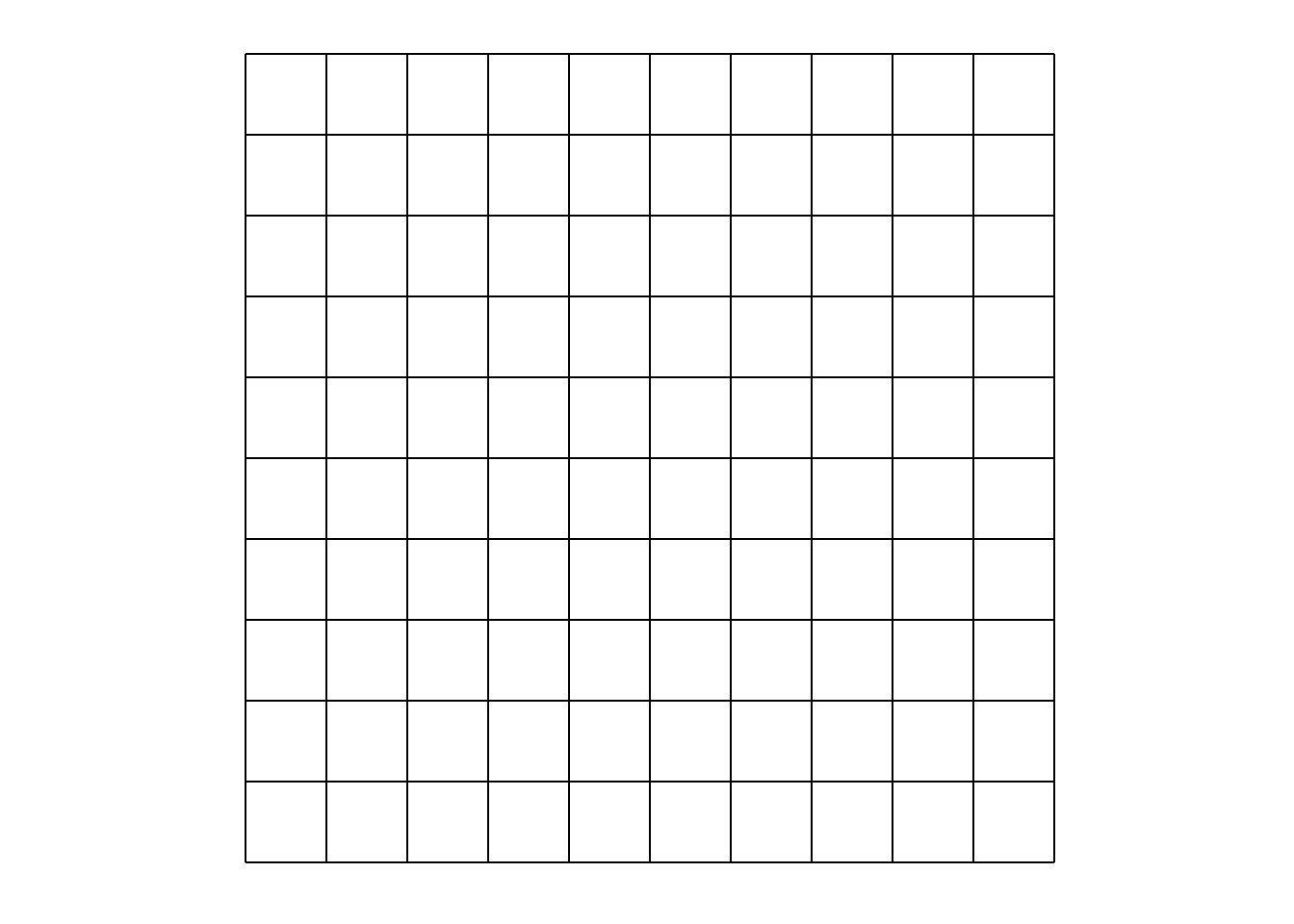

transform_df_coords(): Given dataframe, column names of coordinates⁴, and a transformation matrix, return dataframe with transformed coordinates.

transform_df_coords <- function(df, ..., m = diag(length(df))){
  
  df_names <- names(df)
  
  df_coords <- df %>% 
    select(...)
  
  df_coords_names <- names(df_coords)
  
  df_matrix <- df_coords %>% 
    as.matrix() %>% 
    t()
  
  df_coords_new <- (m %*% df_matrix) %>% 
    t() %>% 
    as_tibble() %>% 
    set_names(df_coords_names)
  
  df_other <- df %>% 
    select(-one_of(df_coords_names))
  
  bind_cols(df_coords_new, df_other) %>% 
    select(df_names)
}

transform_df_coords() is just matrix multiplication, but facilitates applying matrix transformations on a dataframe where each row (in specified columns) represents a vector / coordinate point⁵.

Example in \(\mathbb{R}^2\):

transform_df_coords(tibble(x = 1:4, y = 1:4), x, y, m = matrix(1:4, nrow = 2)) %>% 
  knitr::kable()

x	y
4	6
8	12
12	18
16	24

Again, this is the same as:

\[ \left(\begin{array}{cc} 1 & 3\\ 2 & 4 \end{array}\right) \left(\begin{array}{cc} 1 & 2 & 3 & 4 \\ 1 & 2 & 3 & 4 \end{array}\right) = \left(\begin{array}{cc} 4 & 8 & 12 & 16 \\ 6 & 12 & 18 & 24 \end{array}\right)\]

(Just with a ‘tidy’ dataframe as output.)

Also works with more dimensions, see example in \(\mathbb{R}^3\):

transform_df_coords(tibble(x = 1:5, y = 1:5, z = 1:5), x, y, z, m = matrix(1:9, nrow = 3)) %>% 
  knitr::kable()

x	y	z
12	15	18
24	30	36
36	45	54
48	60	72
60	75	90

However for our visualizations, we only care about examples in 2 dimensions (when we are applying a 2x2 matrix transformation).

Construct objects for graph

For a simple animation I will build dataframes that contain the coordinates for the following objects⁶:

a starting grid and a transformed grid
a starting basis vector and a transformed basis vector

To play nicely with gganimate the start and transformed objects need to have additional properties⁷:

a field that groups like objects across the animation (e.g. id column)
a field that designates transitions between start and transformed states (e.g. time column)

For my example I will be applying the following matrix transformation to our basis vectors⁸. \[ \left(\begin{array}{cc} 0.5 & 0.5\\ 0.5 & -0.25 \end{array}\right)\]

Define transformation matrix:

# same as above examples using `matrix()` but I find inputting into tribble more
# intuitive for 2x2 matrix
transformation_matrix <- tribble(~ x, ~ y,
                                 0.5, 0.5,
                                 0.5, -0.25) %>% 
  as.matrix()

Construct grids:

grid_start <- construct_grid() %>% 
  mutate(id = row_number())

grid_trans <- grid_start %>% 
  # need to `transform_df_coords()` twice as each segment is made up of 2 points
  transform_df_coords(x, y, m = transformation_matrix) %>% 
  transform_df_coords(xend, yend, m = transformation_matrix)

grid_all <- bind_rows(
  mutate(grid_start, time = 1),
  mutate(grid_trans, time = 2)
)

Construct basis vectors:

basis_start <- tibble(
  x = c(0, 0),
  y = c(0, 0),
  xend = c(1, 0),
  yend = c(0, 1),
  # `vec` is unnecessary, will just use to differentiate colors
  vec = c("i", "j")
) %>% 
  mutate(id = nrow(grid_start) + row_number())

basis_trans <- basis_start %>% 
  transform_df_coords(x, y, m = transformation_matrix) %>% 
  transform_df_coords(xend, yend, m = transformation_matrix)

basis_all <- bind_rows(
  mutate(basis_start, time = 1),
  mutate(basis_trans, time = 2)
)

Build visualization

Define breaks in grid:

# If you just want to use the starting grid for the breaks, could do
x_breaks <- unique(grid_start$x)
y_breaks <- unique(grid_start$y)

Define visualization:

p <- ggplot(aes(x = x, y = y, group = id), data = grid_all)+
  geom_segment(aes(xend = xend, yend = yend))+
  geom_segment(aes(xend = xend, yend = yend, colour = vec), data = basis_all, arrow = arrow(length = unit(0.02, "npc")), size = 1.2)+
  scale_x_continuous(breaks = x_breaks, minor_breaks = NULL)+
  scale_y_continuous(breaks = y_breaks, minor_breaks = NULL)+
  coord_fixed()+
  theme_minimal()+
  theme(axis.text = element_blank(),
        axis.title = element_blank(),
        legend.position = "none")

Visualizations

Static image:

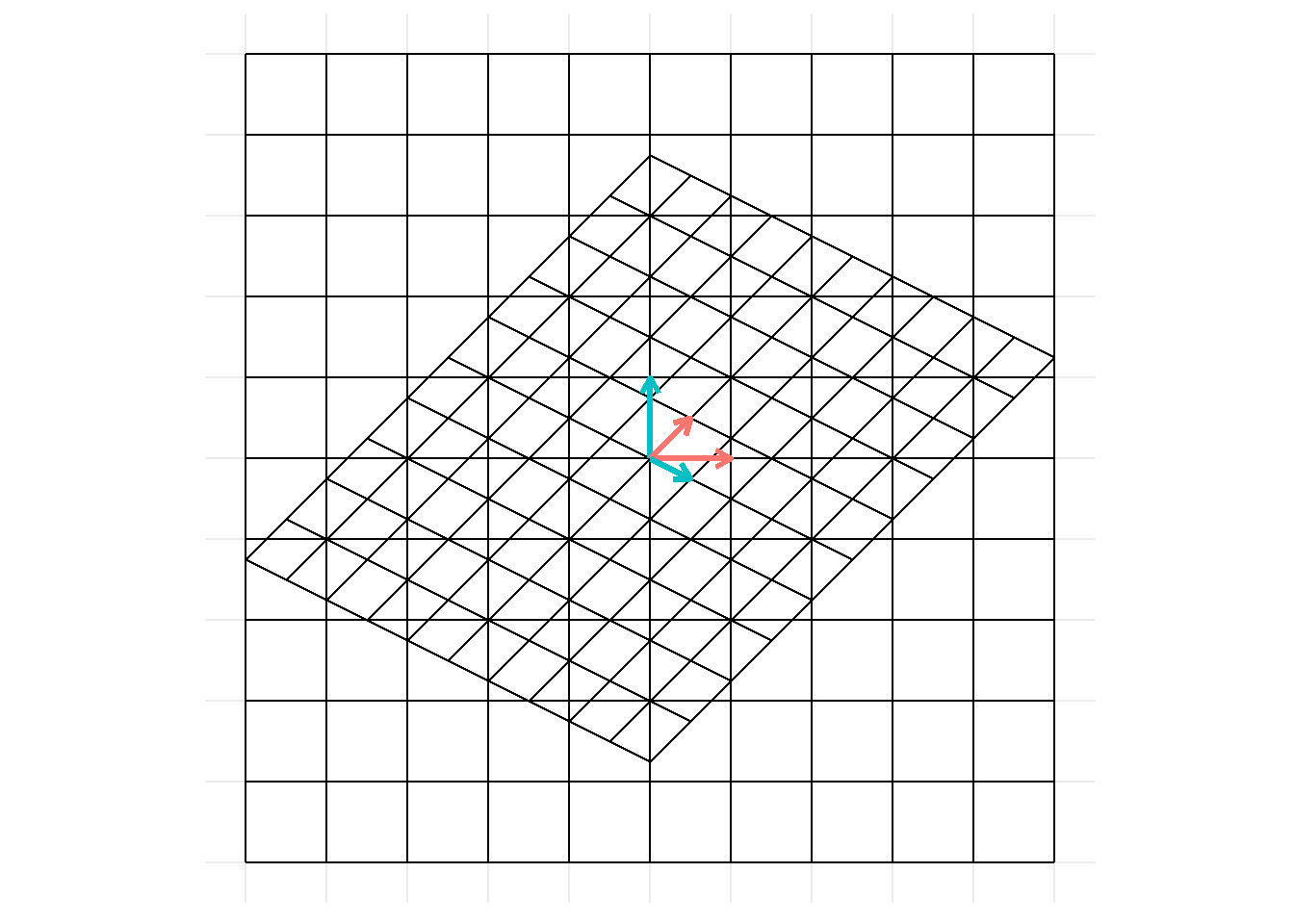
Animation⁹:

p + gganimate::transition_states(time, wrap = FALSE)

And there it is. To view a different matrix transformation, simply change the transformation_matrix defined above and re-run the code chunks¹⁰ or see the Quick start section.

Appendix

The code used to construct images within the appendix is very similar to code already shown¹¹.

On changes

In the few days after sharing this post on 2020-02-20, I made several changes to the images and notes (especially those within the appendix) that I think better clarified points or corrected mistakes.

Multiple matrix transformations

I love how the “Essence of Linear Algebra” series explains how matrix transformations can be thought-of / broken-down sequentially. The same visualization can (kind-of) be set-up here – you just need to add-in an additional layer.

E.g. say, we want to apply a rotation and then a sheer:

rotate_trans <- tribble(~ x, ~ y,
                        cos(pi / 2), -sin(pi / 2),
                        sin(pi / 2), cos(pi / 2)) %>%
  as.matrix()

sheer_trans <- tribble(~ x, ~ y,
                      1, 0,
                      0.5, 1) %>%
  as.matrix()

I.e.

\[\begin{bmatrix} 1 & 0\\ 0.5 & 1 \\ \end{bmatrix} \begin{bmatrix} 0 & -1\\ 1 & 0 \\ \end{bmatrix}X\]

I say kind-of animate these because gganimate transforms coordinates linearly, hence while a transformation may result in a rotation, the in-between states (where gganimate fills in the gaps) will not look like a pure rotation. See Potential improvements for additional notes.

Construct grids:

grid_start <- construct_grid() %>% 
  mutate(id = row_number())

grid_trans <- grid_start %>% 
  # need to `transform_df_coords()` twice as each segment is made up of 2 points
  transform_df_coords(x, y, m = rotate_trans) %>% 
  transform_df_coords(xend, yend, m = rotate_trans)

grid_trans2 <- grid_trans %>% 
  # need to `transform_df_coords()` twice as each segment is made up of 2 points
  transform_df_coords(x, y, m = sheer_trans) %>% 
  transform_df_coords(xend, yend, m = sheer_trans)

grid_all <- bind_rows(
  mutate(grid_start, time = 1),
  mutate(grid_trans, time = 2),
  mutate(grid_trans2, time = 3)
)

Basis vectors:

basis_start <- tibble(
  x = c(0, 0),
  y = c(0, 0),
  xend = c(1, 0),
  yend = c(0, 1),
  # `vec` is unnecessary, will just use to differentiate colors
  vec = c("i", "j")
) %>% 
  mutate(id = nrow(grid_start) + row_number())

basis_trans <- basis_start %>% 
  # need to `transform_df_coords()` twice as each segment is made up of 2 points
  transform_df_coords(x, y, m = rotate_trans) %>% 
  transform_df_coords(xend, yend, m = rotate_trans)

basis_trans2 <- basis_trans %>% 
  # need to `transform_df_coords()` twice as each segment is made up of 2 points
  transform_df_coords(x, y, m = sheer_trans) %>% 
  transform_df_coords(xend, yend, m = sheer_trans)

basis_all <- bind_rows(
  mutate(basis_start, time = 1),
  mutate(basis_trans, time = 2),
  mutate(basis_trans2, time = 3)
)

Define visualization:

p_mult <- ggplot(aes(x = x, y = y, group = id), data = grid_all)+
  geom_segment(aes(xend = xend, yend = yend))+
  geom_segment(aes(xend = xend, yend = yend, colour = vec), data = basis_all, arrow = arrow(length = unit(0.02, "npc")), size = 1.2)+
  scale_x_continuous(breaks = x_breaks, minor_breaks = NULL)+
  scale_y_continuous(breaks = y_breaks, minor_breaks = NULL)+
  coord_fixed()+
  theme_minimal()+
  theme(axis.text = element_blank(),
        axis.title = element_blank(),
        legend.position = "none")

Static image:

p_mult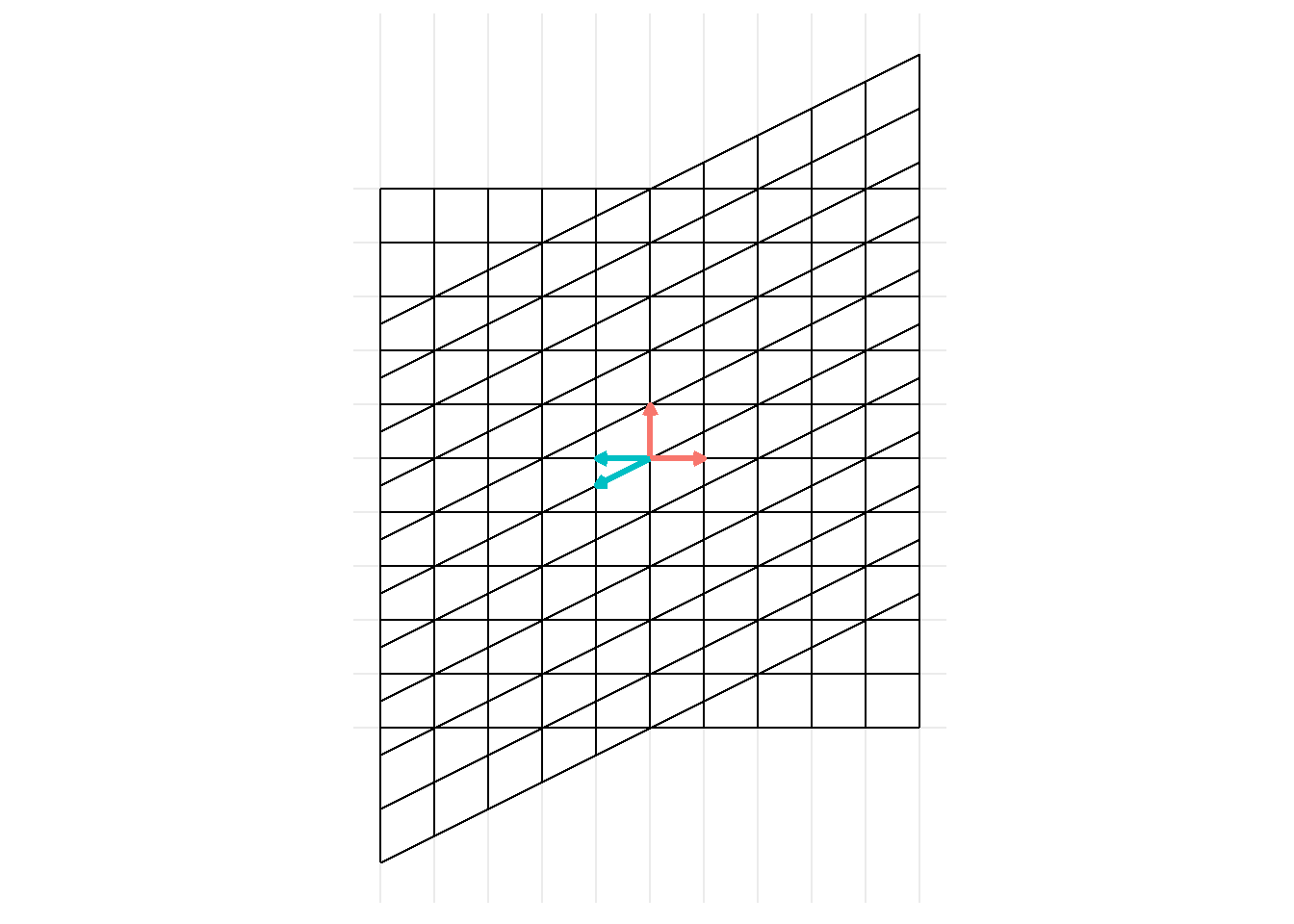

Animation:

p_mult + 
  gganimate::transition_states(time, wrap = FALSE)

Notice that we see the transformations done sequentially. We could also have just inputted the single (simplified) matrix transformation:

\[\begin{bmatrix} -0.5 & -1\\ 1 & 0 \\ \end{bmatrix} X\]

But thinking of the matrix transformations separately can be helpful!

Potential improvements

I have no (current) plans of fleshing this out further. (Though I think a ggplot extension – e.g. ggbasis, gglineartrans – or something could be cool.) In this section I’ll give a few notes regarding short-term things I’d change or fix-up (if I were to keep working on this – maybe I’ll get to a couple of these). Really I should dive into tweenr and transformr packages and associated concepts to get these worked out further.

Problem of squeezing during rotation

You might notice that something about the rotation transformation looks a little off. During the animation, the grid becomes temporarily squished in at some points. We can better see this by placing a circle on the interior of our grid and looking at the rotation of the exterior segments. The exterior segments of the grid should remain tangent to our circle at all points.

circle_df <- tibble(x0 = 0, y0 = 0, r = 5)

p_rotation <- ggplot(aes(), data = filter(grid_all, time <= 2))+
  geom_segment(aes(x = x, y = y, group = id, xend = xend, yend = yend))+
  geom_segment(aes(x = x, y = y, group = id, xend = xend, yend = yend, colour = vec), arrow = arrow(length = unit(0.02, "npc")), size = 1.2, data = filter(basis_all, time <= 2 ))+
  scale_x_continuous(breaks = x_breaks, minor_breaks = NULL)+
  scale_y_continuous(breaks = y_breaks, minor_breaks = NULL)+
  coord_fixed()+
  ggforce::geom_circle(aes(x0 = 0, y0 = 0, r = 5), data = circle_df)+
  theme_minimal()+
  theme(axis.text = element_blank(),
        axis.title = element_blank(),
        legend.position = "none")

p_rotation + gganimate::transition_states(time, wrap = FALSE)

However we can see this doesn’t happen (the grid scrunches up and the exterior segments cut into the circle). The reason this occurs is that during the animation the coordinates follow a straight line path to their new location as explained:

The problem is that coords are tweened linearly which doesn't match a rotation where the tweening should be done on the radians (or, better, tween the transformation matrix instead). There is no support for this in gganimate yet because I haven't figured out the right interface
— Thomas Lin Pedersen (@thomasp85) February 21, 2020

Transformations that you could conceptualize of as rotations will be animated as linear changes to coordinates. As a more extreme example, see animation of a matrix transformation for a \(180^\circ\) rotation:

animate_matrix_transformation(m = matrix(c(-1, 0, 0, 1), nrow = 2))

One fix (irrespective of tweening method in gganimate) could be to set specific coordinates at each frame (so that the lack of a true rotation wouldn’t be noticable)¹².

Problem of jittery points during rotation

Beyond the squishing, it appears coordinate points (added via geom_point()) also look a little jittery during rotations.

For example:

points_start <- crossing(x = c(-3.5:3.5), y = c(-3.5:3.5)) %>% 
  mutate(id = nrow(grid_start) + nrow(basis_start) + row_number())
 
points_trans <- points_start %>% 
  transform_df_coords(x, y, m = rotate_trans)

points_all <- bind_rows(
  mutate(points_start, time = 1),
  mutate(points_trans, time = 2))

p_points <- p +
  geom_point(data = points_all, colour = "royalblue3")

p_points + gganimate::transition_states(time, wrap = FALSE)

# maybe just my eyes... maybe need to increase framerate... or something

p_points <- p_rotation +
  geom_point(aes(x, y), data = points_all, colour = "royalblue3")

p_points + gganimate::transition_states(time, wrap = FALSE)

Miscellaneous notes

I could not figure out how to add multiple polygons via geom_polygon() in a way that kept smooth transitions¹³. Would likely need to explore tweenr, transformr….
Would be nice to add title of image as the matrix transformation being conducted¹⁴
May be better to render to video (rather than gif) so could pause to view
In general, could make more elegant / sophisticated… especially regarding how transformations are applied across layers
- Would be nice if was set-up to apply the transformations across all (or specified layers).

Note on scales

May want to make breaks extend across entire range (rather than just over x, y ranges of grid_start).

Expand breaks in scales:

x_breaks <-
  seq(
    from = 
      floor(min(c(grid_all$x, grid_all$xend))), 
    to = 
      ceiling(max(c(grid_all$x, grid_all$xend))), 
    by = 1)

y_breaks <-
  seq(
    from = 
      floor(min(c(grid_all$y, grid_all$yend))), 
    to = 
      ceiling(max(c(grid_all$y, grid_all$yend))), 
    by = 1)

Which are shown throughout the series and most notably in chapters 3 and 13.↩︎
See section [Problems and potential improvements] for notes on a couple potential updates I’ll make… not positive I’ll keep the gist code updated.↩︎
And may not care about understanding how to do multiple transformations, adding additional layers, etc.↩︎
/ vectors↩︎
I’m guessing there is a better / more elegant function already out there for ‘tidy matrix multiplication’ or something… but couldn’t immediately think of anything.↩︎
You could add additional objects to the image – just need to ensure you create start and transformed versions of each object.↩︎
Creating these is not needed if you just wanted to create static images for the below examples.↩︎
No real reason for choosing this transformation, just thought it looked cool.↩︎
If wrap = TRUE (default) the reverse looping of the image is inaccurate as the transformation back to the original basis actually represents a transformation by the inverse of the transformation matrix. Though leaving it in would look cooler.↩︎
Could functionalize more… or make a shiny app, or do more with, see [Problems and potential improvements] for notes…↩︎
Can largely skim over↩︎
Though this gets into decomposing the rotation, etc. components of the matrix transformation of interest for each frame.↩︎
Seems issue has to do with group needing to apply both to the polygon at a given time as well as points on the polygon across time.↩︎
Would require latex title which I don’t know if is supported by gganimate↩︎

Visualizing Matrix Transformations